EECS 442: Computer Vision (Winter 2024)

Homework 1 – Numbers and Images

Instructions

This homework is due at 11:59 p.m. on Wednesday January 31st, 2024.

The submission includes two parts:

1. To Canvas: submit a zip file containing a single directory with your uniqname as the name that contains all your code (subdirectories are fine).

   - We have indicated questions where you have to do something in code in red. If gradecope asks for it, also submit your code in the report with the formatting below.

   Starter code is given to you on Canvas under the “Homework 1” assignment. You can also download it here. Clean up your submission to include only the necessary files.

   Submission Tip: Use the Tasks Checklist and Canvas Submission Checklist at the end of this homework. We also provide a script that validates the submission format here.

2. To Gradescope: submit a pdf file as your write-up, including your answers to all the questions and key choices you made.

   - We have indicated questions where you have to do something in the report in green. Some coding questions also need to be included in the report.

   The write-up must be an electronic version. No handwriting, including plotting questions. \(\LaTeX\) is recommended but not mandatory.

   For including code, do not use screenshots. Generate a PDF using a tool like this or using this Overleaf LaTeX template. If this PDF contains only code, be sure to append it to the end of your report and match the questions carefully on Gradescope.

Python Environment

Consider referring to the Python standard library docs when you have questions about Python utilties.

We recommend you install the latest Anaconda for Python 3.12. This is a Python package manager that includes most of the modules you need for this course. We will make use of the following packages extensively in this course:

• Numpy
• Matplotlib
• OpenCV

Overview

In this assignment, you’ll work through three tasks that help set you up for success in the class as well as a short assignment involving playing with color. The assignment has three goals.

1. Show you bugs in a low-stakes setting. You’ll encounter a lot of programming mistakes in the course and we want to show you common bugs early on. Here, the programming problems are deliberately easy!
2. Learn to write reasonably good Python and NumPy code. Having layers of nested for loops will cause bugs and is not feasible for us to debug, use NumPy effectively! If you have not had any experience with NumPy, read this tutorial before starting.

The assignment has four parts and corresponding folders in the starter code:

• Numpy Intro (folder numpy/)
• Data Interpretation and Visualization (folder visualize/)
• Lights on a Budget (folder dither/)
• Colorspaces

Numpy Intro

All the code/data for this is located in the folder numpy/. Each assignment requires you to fill in the blank in a function (in tests.py and warmup.py) and return the value described in the comment for the function. There’s driver code you do not need to read in run.py and common.py.

Note: All the python below refer to python3. As we stated earlier, we are going to use Python 3.12 in this assignment. Python 2 was sunset on January 1, 2022.

1. (40 points) Fill in the code stubs in tests.py and warmups.py. Put the terminal output in your pdf from:

$ python run.py --allwarmups
$ python run.py --alltests

Do I have to get every question right? We give partial credit: each warmup exercise is worth 2% of the total grade for this question and each test is worth 3% of the total grade for this question.

Tests Explained

When you open one of these two files, you will see starter code that looks like this:

def sample1(xs):
	"""
	Inputs:
	- xs: A list of values
	Returns:
	The first entry of the list
	"""
	return None

You should fill in the implementation of the function, like this:

def sample1(xs):
	"""
	Inputs:
	- xs: A list of values
	Returns:
	The first entry of the list
	"""
	return xs[0]

You can test your implementation by running the test script:

python run.py --test w1     # Check warmup problem w1 from warmups.py
python run.py --allwarmups  # Check all the warmup problems
python run.py --test t1     # Check the test problem t1 from tests.py
python run.py --alltests    # Check all the test problems

# Check all the warmup problems; if any of them fail, then launch the pdb
# debugger so you can find the difference
python run.py --allwarmups --pdb

If you are checking all the warmup problems (or test problems), the perfect result will be:

python run.py --allwarmups
Running w1
Running w2
...
Running w20
Ran warmup tests
20/20 = 100.0

Warmup Problems

You need to solve all 20 of the warmup problems in warmups.py. They are all solvable with one line of code.

Test Problems

You need to solve all 20 problems in tests.py. Many are not solvable in one line. You may not use a loop to solve any of the problems, although you may want to first figure out a slow for-loop solution to make sure you know what the right computation is, before changing the for-loop solution to a non for-loop solution. The one exception to the no-loop rule is t10 (although this can also be solved without loops).

Here is one example:

def t4(R, X):
	"""
	Inputs:
	- R: A numpy array of shape (3, 3) giving a rotation matrix
	- X: A numpy array of shape (N, 3) giving a set of 3-dimensional vectors
	Returns:
	A numpy array Y of shape (N, 3) where Y[i] is X[i] rotated by R
	Par: 3 lines
	Instructor: 1 line
	Hint:
	1) If v is a vector, then the matrix-vector product Rv rotates the vector
	   by the matrix R.
	2) .T gives the transpose of a matrix
	"""
	return None

What We Provide

For each problem, we provide:

• Inputs: The arguments that are provided to the function
• Returns: What you are supposed to return from the function
• Par: How many lines of code it should take. We don’t grade on this, but if it takes more lines than this, there is probably a better way to solve it. Except for t10, you should not use any explicit loops.
• Instructor: How many lines our solution takes. Can you do better? Hints: Functions and other tips you might find useful for this problem.

Walkthroughs and Hints

Test 8: If you get the axes wrong, numpy will do its best to make sure that the computations go through but the answer will be wrong. If your mean variable is \(1 \times 1\), you may find yourself with a matrix where the full matrix has mean zero. If your standard deviation variable is \(1 \times M\), you may find each column has standard deviation one.

Test 9: This sort of functional form appears throughout data-processing. This is primarily an exercise in writing out code with multiple nested levels of calculations. Write each part of the expression one line at a time, checking the sizes at each step.

Test 10: This is an exercise in handling weird data formats. You may want to do this with for loops first.

1. First, make a loop that calculates the vector C[i] that is the centroid of the data in Xs[i]. To figure out the meaning of things, there is no shame in trying operations and seeing which produce the right shape. Here we have to specify that the centroid is M-dimensions to point out how we want Xs[i] interpreted. The centroid (or average of the vectors) has to be calculated with the average going down the columns (i.e., rows are individual vectors and columns are dimensions).
2. Allocate a matrix that can store all the pairwise distances. Then, double for loop over the centroids i and j and produce the distances.

Test 11: You are given a set of vectors \(\xB_1, \ldots, \xB_N\) where each vector \(x_i \in \mathbb{R}^M\). These vectors are stacked together to create a matrix \(\XB \in \mathbb{R}^{N \times M}\). Your goal is to create a matrix \(\DB \in \mathbb{R}^{N \times N}\) such that \(\DB_{i,j} = \|\xB_i - \xB_j\|\). Note that \(\|\xB_i - \xB_j\|\) is the L2-norm or the Euclidean length of the vector. The useful identity you are given is that \(\|\xB-\yB\|^2 = \|\xB\|^2 + \|\yB\|^2 - 2\xB^T \yB\). This is true for any pair of vectors \(\xB\) and \(\yB\) and can be used to calculate the distance quickly.

At each step, your goal is to replace slow but correct code with fast and correct code. If the code breaks at a particular step, you know where the bug is.

1. First, write a correct but slow solution that uses two for loops. In the inner body, you should plug in the given identity to make \(\DB_{i,j} = \|\xB_i\|^2 + \|\xB_j\|^2 - 2 \xB_i^T \xB_j\). Do this in three separate terms.
2. Next, write a version that first computes a matrix that contains all the dot products, or \(\PB \in \mathbb{R}^{N \times N}\) such that \(\PB_{i,j} = \xB_i^T \xB_j\). This can be done in a single matrix-matrix operation. You can then calculate the distance by doing \(\DB_{i,j} = \|\xB_i\|^2 + \|\xB_j\|^2 - 2\PB_{i,j}\).
3. Finally, calculate a matrix containing the norms, or a \(\NB \in \mathbb{R}^{N \times N}\) such that \(\NB_{i,j} = \|\xB_i\|^2 + \|\xB_j\|^2\). You can do this in two stages: first, calculate the squared norm of each row of \(\XB\) by summing the squared values across the row. Suppose \(\SB\) is this array (i.e., \(\SB_{i} = \|\xB_i\|^2\) and \(\SB_{i} \in \mathbb{R}^{N}\)), but be careful that you look at the shape that you get as output. If you compute \(\SB + \SB^T\), you should get \(\NB\). Now you can calculate the distance inside the double for loop as \(\DB_{i,j} = \NB_{i,j} - 2 \PB_{i,j}\).
4. The double for loop is now not very useful. You can just add/scale the two arrays together elementwise.

Test 18: Here you draw a circle by finding all entries in a matrix that are within \(r\) cells of a row \(y\) and column \(x\). This is a not particularly intellectually stimulating exercise, but it is practice in writing (and debugging) code that reasons about rows and columns.

1. First, write a correct but slow solution that uses two for loops. In the inner body, plug in the correct test for the given i, j. Make sure the test passes; be careful about rows and columns.
2. Look at the documentation for np.meshgrid briefly. Then call it with np.arange(3) and np.arange(5) as arguments. See if you can create two arrays such that IndexI[i,j] = i and IndexJ[i,j] = j.
3. Replace your test that uses two for loops with something that just uses IndexI and IndexJ.

Data Interpretation and Visualization

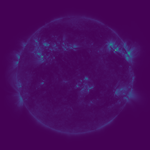
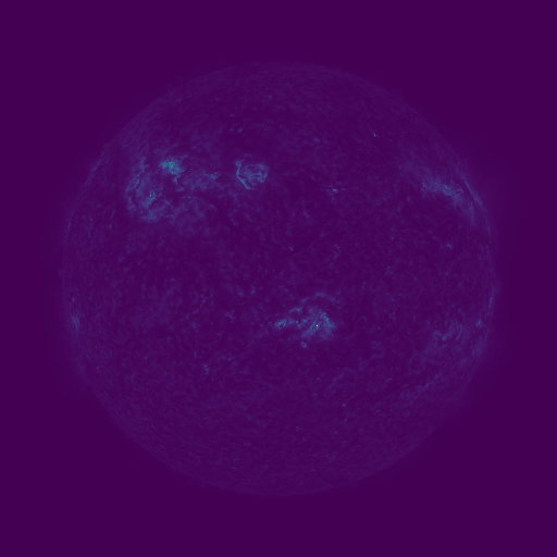
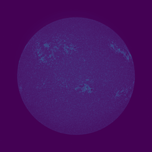
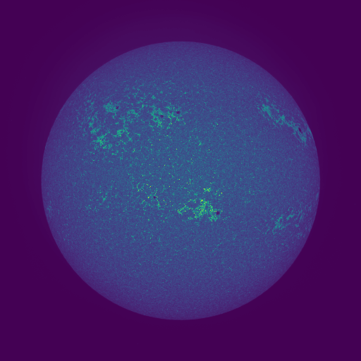
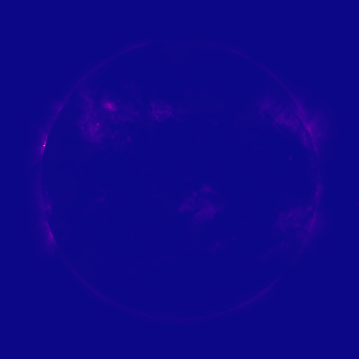
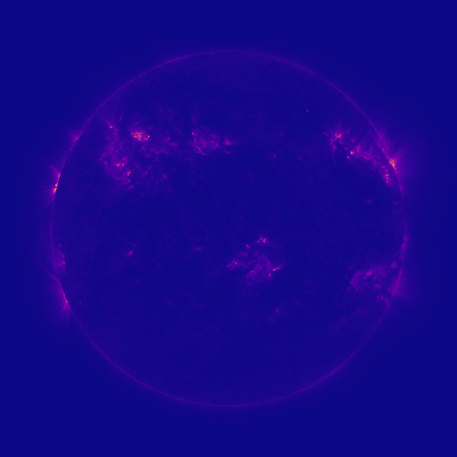
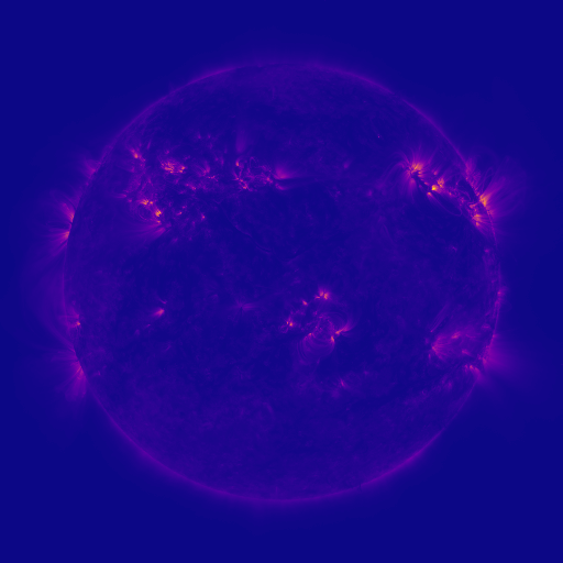
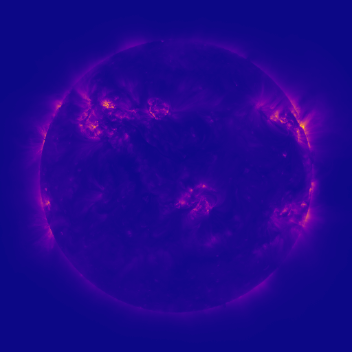
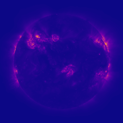
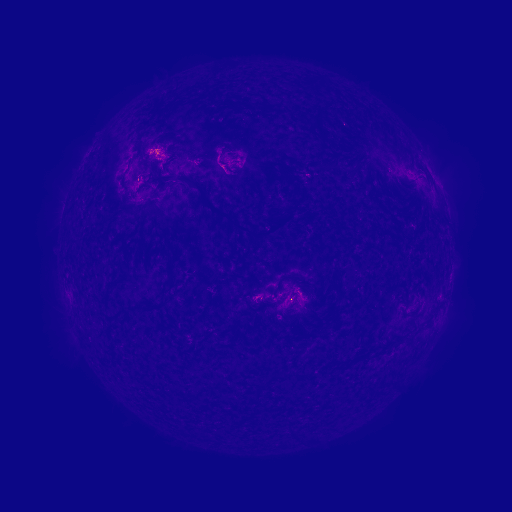
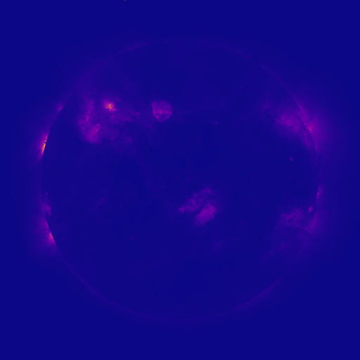
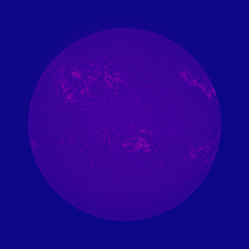
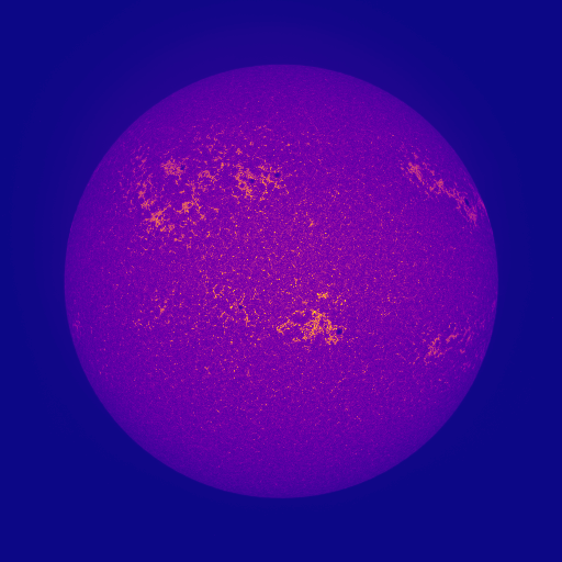
Throughout the course, a lot of the data you have access to will be in the form of an image. These won’t be stored and saved in the same format that you’re used to when interacting with ordinary images, such as off your cell phone: sometimes they’ll have negative values, really really big values, or invalid values. If you can look at images quickly, then you’ll find bugs quicker. If you only print debug, you’ll have a bad time. To teach you about interpreting things, I’ve got a bunch of mystery data that we’ll analyze together. You’ll write a brief version of the important imsave function for visualizing.

Let’s load some of this mysterious data.

>>> X = np.load("mysterydata/mysterydata.npy")
>>> X
array([[[0, 0, 0, ..., 0, 0, 1],
		[0, 0, 0, ..., 0, 0, 0],
		[0, 0, 0, ..., 0, 0, 0],
		...,
		[0, 0, 0, ..., 0, 0, 0],
		[0, 0, 0, ..., 0, 0, 0],
		[0, 0, 0, ..., 0, 0, 0]],

	   ... (some more zeros) ...

	   [[0, 0, 0, ..., 0, 0, 0],
		[0, 0, 0, ..., 0, 0, 0],
		[0, 0, 0, ..., 0, 0, 0],
		...,
		[0, 0, 0, ..., 0, 0, 0],
		[0, 0, 0, ..., 0, 0, 0],
		[0, 0, 0, ..., 0, 0, 0]]], dtype=uint32)

Looks like it’s a bunch of zeros. Nothing to see here folks! For better or worse: Python only shows the sides of an array when printing it and the sides of images that have gone through some processing tend to not be representative.

After you print it out, you should always look at the shape of the array and the data type.

>>> X.shape
(512, 512, 9)
>>> X.dtype
dtype('uint32')

The shape and datatype are really important. If something is an unexpected shape, that’s really bad. This is similar to doing a physics problem where you’re trying to measure the speed of light (which should be in m/s), and getting a result that is in gauss. The computer may happily chug along and produce a number, but if the units or shape are wrong, the answer is almost certainly wrong. The datatype is also really important, because data type conversion can be lossy: if you have values between 0 and 1, and you convert to an integer format, you’ll end up with 0s and 1s.

In this particular case, the data has height 512 (the first dimension), width 512 (the second), and 9 channels (the last). These order of dimensions here is a convention, meaning that there are multiple equivalent options. For instance, in other conventions, the channel is the first dimension. Generally, you’ll be given data that is \(HxWxC\) and we’ll try to be clear about how data is stored. If later on, you’re given some other piece of data, figuring out the convention is a bit like rotating a picture until it looks right: figure out what you expect, and flip things until it looks like you’d expect.

If you’ve got an image, after you print it, you probably want to visualize the output.

We don’t see in 9 color channels, and so you can’t look at them all at once. If you’ve got a bug, one of the most important things to do is to look at the image. You can look at either the first channel or all of the channels as individual images.

>>> plt.imsave("vis.png",X[:,:,0])

You can see what the output looks like in Figure 1. This is a false color image. Given the image, you want to find the minimum value (vmin) and the maximum value (vmax) and assign colors based on where each pixel’s value falls between those. These colors look like: Low High. plt.imsave finds vmin and vmax for you on its own by computing the minimum and maximum of the array.

If you’d like to look at all 9 channels, save 9 images:

>>> for i in range(9):
...     plt.imsave("vis_%d.png" % i,X[:,:,i])

If you’re inside a normal python interpreter, you can do a for loop. If you’re inside a debugger, it’s sometimes hard to do a for loop. If you promise not to tell your programming languages friends, you can use side effects to do a for loop to save the data.

(Pdb) [plt.imsave("vis_%d.png" % i,X[:,:,i]) for i in range(9)]
[None, None, None, None, None, None, None, None, None]

The list of Nones is just the return value of plt.imsave, which saves stuff to disk and returns a None.

If you’d like to change the colormap, you can specify this with cmap. For instance,

>>> for i in range(9):
...     plt.imsave("vis_%d.png" % i,X[:,:,i],cmap='plasma')

produces the outputs in Figure 2. These use the plasma colormap which looks like: Low High.

Pixel Value Ranges

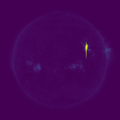
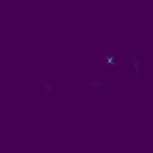
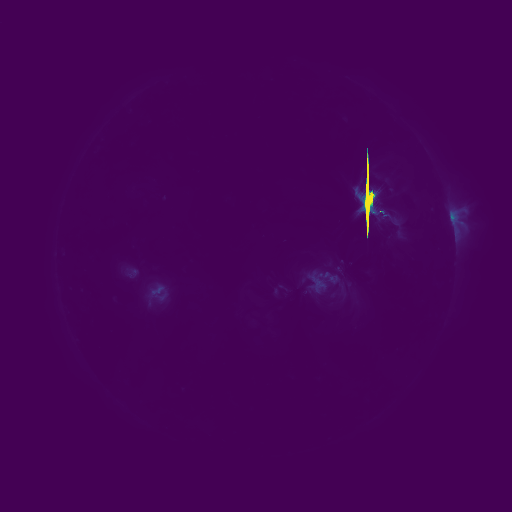
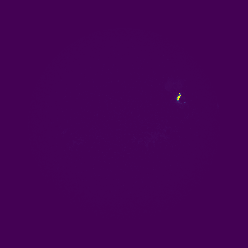
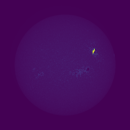
1. (2 points) Try loading mysterydata2.npy and visualizing it. You should get something like Figure 3. It’s hard to see stuff because one spot is really bright. In this case, it’s because there’s a solar flare that’sproducing immense amounts of light. A common trick for making things easier to see is to apply a nonlinear correction. Here are a few options:

   \[p^\gamma \ \textrm{with}\ \gamma \in [0,1] \quad\textrm{or}\quad \log(p) \quad\textrm{or}\quad \log(1+p)\]

   where the last one can be done with np.log1p. Apply a nonlinear correction to the second mystery data and visualize it. Put two of the channels i.e. X[:,:,i] as images into the report. You can stick them side-by-side.

Invalid Pixel Values

Let’s try this again, using one of the other data.

>>> X = np.load("mysterydata/mysterydata3.npy")
>>> for i in range(9):
...     plt.imsave("vis3_%d.png" % i,X[:,:,i])

The results are shown in Figure 4. They’re all white. What’s going on?

If you’ve got an uncooperative piece of data that won’t visualize or produces buggy results, it’s worth checking to see if all the values are reasonable. One option that’ll cover all your cases is np.isfinite, which is False for values that are NaN (not a number) or \(\pm \infty\) and True otherwise. If you then take the mean over the array, you get the fraction of entries that are normal-ish. If the mean value is anything other than 1, you may be in trouble. Here:

>>> np.mean(np.isfinite(X))
0.6824828253851997

Alternatively, this also works:

>>> np.sum(~np.isfinite(X))
749117

Other things that check things are np.isnan (which returns True for NaNs) and np.isinf (which returns True for infinite values). Even a single NaN in your data is a problem: any number that touches another NaN turns into a NaN. The totally white values happen because plt.imsave tries to find vmin/vmax, and the minimum of a value and a NaN is a NaN. The resulting color is a NaN as well. If you’ve got NaNs in your data, many functions you may want to use (e.g., mean, sum, min, max, median, quantile) have a “nan” version.

2. (2 points) Fix the images by determining the right range (use np.nanmin, np.nanmax) and then pass arguments into plt.imsave to set the range for the visualization. To figure out what arguments to set, look at the documentation for plt.imsave. Put two images from mysterydata3.npy in the report.

Rolling Your Own plt.imsave

You’ll make your own plt.imsave by filling in colormapArray. Here’s how the false color image works: You’re given a \(H \times W\) matrix \(X\) and a colormap matrix \(C\) that is \(N \times 3\) where each row is a color red/green/blue. You produce a \(H \times W \times 3\) matrix \(O\). Each scalar-valued pixel \(X[i,j]\) gets converted into red/green/blue values for \(O[i,j,:]\) following this rule: if the pixel has value \(v\) the corresponding output color comes from a row determined by (approximately)

However, you’ll have to be very careful – this precise equation won’t always work. As an exercise – can you spot something that might cause the expression to be a NaN?

3. (3 points) Fill in colormapArray. To test, you’ll have to write some calling code in the main part. You can use either plt.imsave or cv2.imwrite to save the image to an file. Include source code in the report.

4. (3 points) Visualize mysterydata4.npy using your system without it crashing and put all nine images into your report. You may have to make a design decision about what to do about results that are undefined. If the results are undefined, then any option that seems reasonable is fine. Your colormap should look similar to Figure 2. If the colors look inverted, see Beware 3!

Lights on a Budget

The code and data for this are located in dither/. This contains starter code dither.py, an image gallery gallery/. Some of these images are very high resolution, so we are providing a copied that has been downsampled to be \(\le 200\) pixels in gallery200/. We’re also providing sample outputs for all algorithms in bbb/.

While modern computer screens are typically capable of showing 256 different intensities per color (leading to \(256^3 = 16.7\) million possible color combinations!) this wasn’t always the case. Many types of displays are only capable of showing a smaller number of light intensities. Similarly, some image formats cannot represent all \(256^3\) colors: GIFs, for instance, can only store 256 colors.

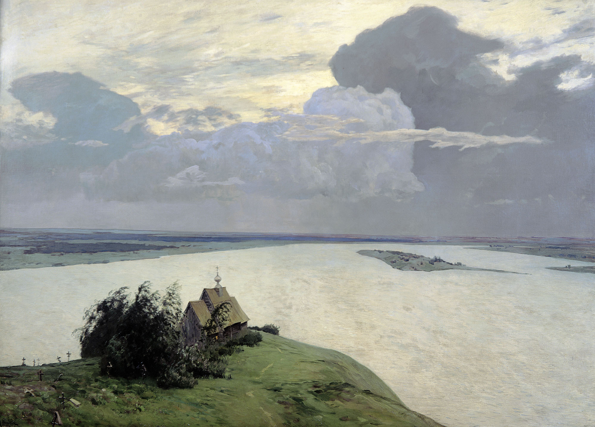
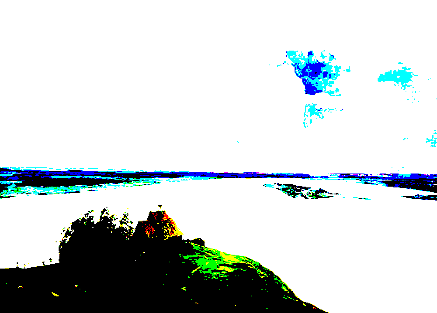
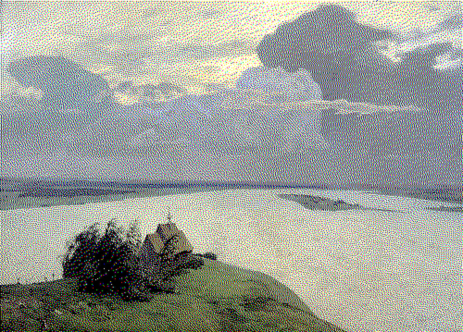
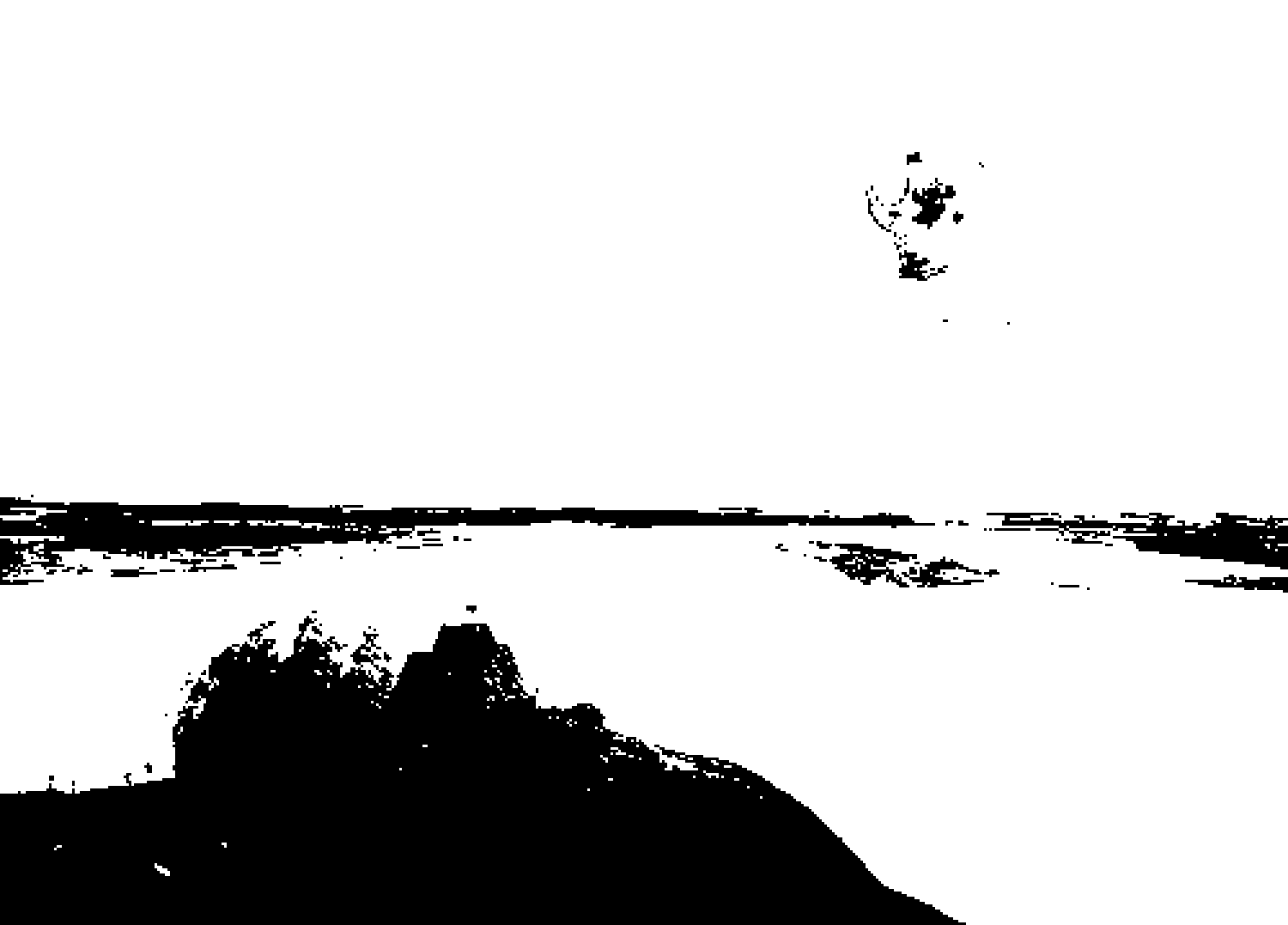
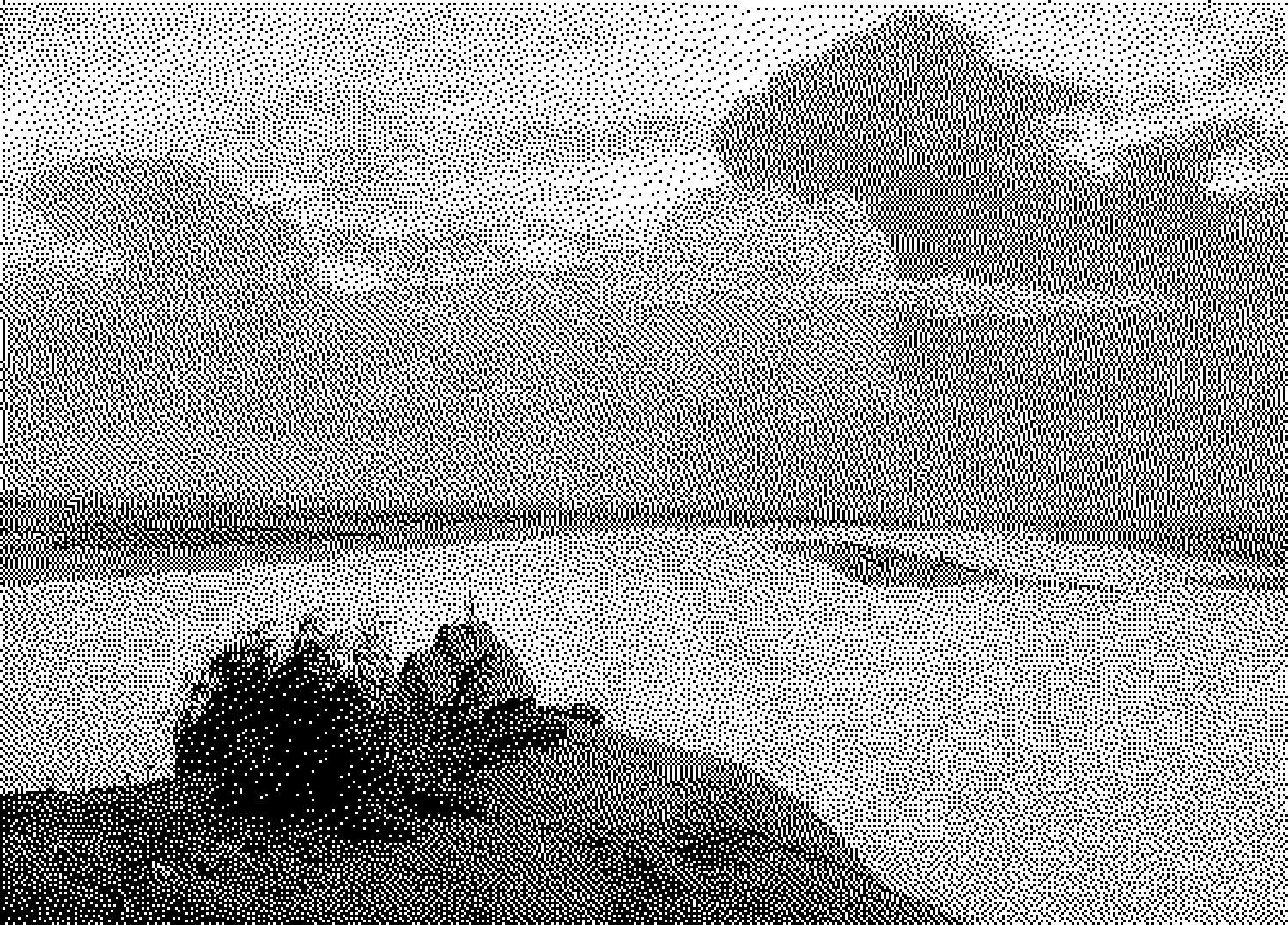
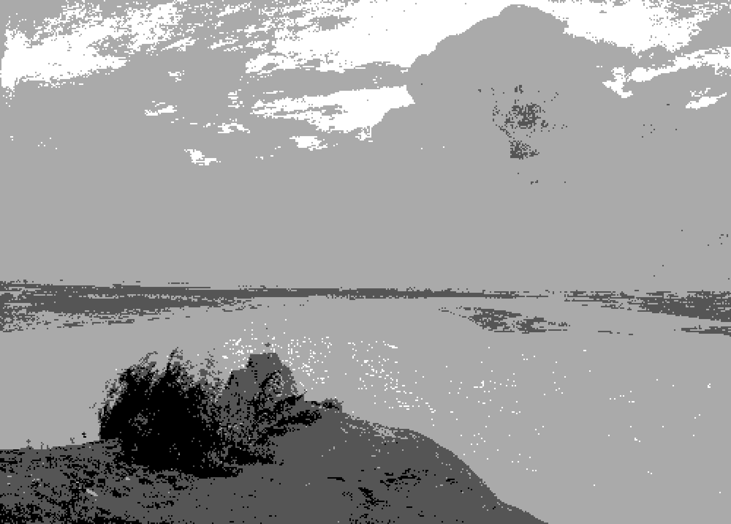
You’ll start out with a full byte of data to work with and will be asked to represent the image with a smaller number of bits (typically 1 or 2 bits per pixel).

Input: As input the algorithm will get:

1. A \(H \times W\) floating point image with brightness ranging from 0 to 1, and
2. A palette consisting of all the \(K\) allowed brightness settings (each floats in the range 0 to 1).

Output: As output, each algorithm produces a \(H \times W\) uint8 image with brightness ranging from \(0\) to \(K-1\).

We’ll call this a quantized image. You can take the palette and the quantized image and make a new image via ReconstructedImage[y,x] = Palette[QuantizedImage[y,x]]. Note that the array you get from numpy will get be indexed by y (or row) first and then by x (or column). The goal of the algorithm is to find a quantized image such that it is close to the reconstructed image. While this doesn’t technically save us space if implemented naively, we could further gain savings by using \(\log_2(K)\) bits rather than the \(8\) bits.

The Rest of the Homework: You’ll build up to Floyd-Steinberg Dithering. You’ll:

1. Start with a really naive version;
2. Do Floyd-Steinberg;
3. Add a resize feature to the starter code;
4. Handle color;
5. (optionally) Handle funny stuff about how monitors display outputs.

Naive Approach

The simplest way to make an image that’s close is to just pick the closest value in the palette for each pixel.

1. (10 points) 2 coding, 3 report questions.

   1. First, fill in quantize(v,palette) in the starter code.

      This should return the index of the nearest value in the palette to the single value v. Note that we’re making this general by letting it take a palette. For speed this would normally done by pre-selecting a palette where the nearest entry could be calculated fast. Do this without a for-loop. Look at np.argmin. Indeed, the beauty of the Internet is that if you search for “numpy find index of smallest value”, you’ll likely find this on your own. In general, you should feel free to search for numpy documentation or for whether there are functions that will make your life easier.

   2. (2 points) Second, fill in quantizeNaive(IF,palette) in the starter code. Include source code in the report.

      This takes a floating point image of size HxW and a palette of values. Create a new uint8 matrix and use quantize() to find the index of the nearest pixel. Return the HxW uint8 image containing the palette indices (not values!). Once you’ve done this, you can call python dither.py gallery200 results quantizeNaive to see the results. Open up view.htm. You can sort of recognize the images, but this is not an aesthetically pleasing result. If you change --numbits you can control the size of the palette.

      Beware:

      At this stage, many people naturally want to do something like output = IF, which gives you an array that’s as big as the input. Keep in mind that when you get IF as an argument, you are getting a reference/address/pointer! If you modify that variable, the underlying data changes.

      Allocate a new matrix via output = np.zeros(IF.shape,dtype=np.uint8). Otherwise, this is like asking to copy your friends’ notes, and then returning them with doodles all over them.

   3. (2 points) If you apply this to the folder gallery, why might your code (that calls quantize) take a very long time? (1 sentence)

   4. (2 points) Pause the program right after algoFn (the function for your dithering algorithm) gets called. Visualize the values in the image with plt.imsave or plt.imshow. These produce false color images. The default colormap in matplotlib looks like: Low High. You should notice that something is different about the intensity values after they’ve been converted to the palette.

      Do low intensity values correspond to low palette values? Explain (1 sentence) what’s going on. You may have to look through the code you’re given (a good habit to get into).

   5. (4 points) Put two results of inputs from gallery and corresponding outputs in your answer document. Use aep.jpg plus any other one that you like. While you can play with --num-bits to get a sense of how things work, you should have --num-bits set to 1 for the output.

Floyd-Steinberg

Naively quantizing the image to a palette doesn’t work. The key is to spread out the error to neighboring pixels. So if pixel (i,j) is quantized to a value that’s a little darker, you can have pixel (i,j+1) and (i+1,j) be brighter. Your job is next to implement quantizeFloyd, or Floyd-Steinberg Dithering. The pseudocode from Wikipedia (more or less) is below (updated to handle the fact that we’re returning the index):

# ... some calling code up here ..
# you'll have to set up pixel
output = new HxW that indexes into the palette
for y in range(H): for x in range(W):
	oldValue = pixel[x][y]
	colorIndex = quantize(oldValue,palette)
	# See Beware 1! re: rows/columns
	output[x][y] = colorIndex
	newValue = palette[colorIndex]
	error = oldValue-newValue
	pixel[x+1][y]   += error*7/16
	pixel[x-1][y+1] += error*3/16
	pixel[x][y+1]   += error*5/16
	pixel[x+1][y+1] += error*1/16
return output

2. (8 points) 1 coding, 2 report questions.

   1. Implement Floyd-Steinberg Dithering in quantizeFloyd.

      Beware:

      1. Different programs, libraries, and notations will make different assumptions about whether x or y come first, and whether the image is height \(\times\) width or width \(\times\) height.

      2. This algorithm, like most image processing algorithms, has literal edge cases. Keep it simple, no need to be fancy.

      3. In Python, objects like lists, dictionaries, and NumPy arrays are passed by reference!

   2. (2 points) In your own words (1-2 sentences), why does dithering (the general concept) work? Try stepping back from your computer screen or, if you wear glasses, take them off.

   3. (6 points) Run this on gallery. Put three results in your document, including aep.jpg. Don’t adjust --num-bits and use the defaults.

Resizing Images

We provided you with two folders of images, gallery/ and gallery200/. The images in gallery200 are way too small; the images in gallery are way too big! Giving you the images in all sizes would be too big, so it would be ideal if we could resize images to some size we decide when we run the program.

3. (2 points) 1 coding question.

   1. Fill in resizeToSquare(I,maxDim). Include source code in the report.

      If the input image is smaller than maxDim on both sides, leave it alone; if it is bigger, resize the image to fit inside a maxDim by maxDim square while keeping the aspect ratio the same (i.e., the image should not stretch). Use the opencv function cv2.resize (and refer to documentation). You can now resize to your hearts content using the --resizeto flag.

Handling Color

You’ve written a version of dithering that handles grayscale images. Now you’ll write one that handles color.

4. (20 points) 2 coding, 1 report questions.

   1. (4 points) Rewrite quantize(v,palette) so that it can handle both scalar v and vector v. Include source code in the report.

      If v is a n-dimensional vector it should return a set of n vector indices (i.e., for each element, what is the closest value in the palette). You can use a for loop, but remember that: (a) broadcasting can take a M-dimensional vector and N-dimensional vector and produce a MxN dimensional matrix; and (b) many functions have an axis argument. If you are given a vector, don’t overwrite individual elements of it either!

   2. (8 points) Make sure that your version of quantizeFloyd(IF,palette) can handle images with multiple channels. Include source code in the report.

      You may not have to do anything. If IF is a \(H \times W \times 3\) array, IF[i,j] refers to the 3D vector at the i,jth pixel i.e., [IF[i,j,0],IF[i,j,1],IF[i,j,2]]. You can add and subtract that vector however you want.

      Beware: When you get v = IF[i,j], you are getting a reference/address/pointer!

   3. (8 points) Generate any four results of your choosing in color. This can be on the images we provide or on some other image you’d like. Put them in your document. For your submission, don’t adjust --num-bits, use the default value of 1. Set the grayscale flag to 0.

(Optional) Gamma Correction

If you look at your outputs from a distance (unless you crank up the number of bits used), you’ll notice they’re quite a bit brighter! This is a bit puzzling. As a sanity check, you can check the average light via np.mean(reconstructed) and np.mean(original). They should be about the same.

The amount of light your monitor sends out isn’t linearly related to the value of the image. In reality, if the image has a value \(v \in [0,1]\), the monitor actually shows something like \(v^\gamma\) for \(\gamma = 2.4\) (for most values, except for some minus some technicalities near 0 – see sRGB on Wikipedia). This is because human perception isn’t linearly related to light intensity and storing the data pre-exponent makes better use of a set of equally-spaced values. However, this messes with the algorithm’s assumptions: suppose the algorithm reconstructs two pixels which are both \(0.5\) as a pixel with a \(0\) and one with a \(1\). The total amount of light that comes off the screen is \(2 * 0.5^{2.4} \approx 0.379\) and \(0 + 1^{2.4} = 1\). They’re not the same! Oof.

The solution is to operate in linear space. You can convert between linear and sRGB via linearToSRGB and SRGBToLinear. First convert the image from sRGB to linear; whenever you want to quantize, convert the linear value back to SRGB and find the nearest sRGB value in the palette; when you compute the error, make sure to convert the new value back to linear.

You should feel free to use the outputs from this implementation for your chosen result.

Colorspaces

The same color may look different under different lighting conditions. Images rubik/indoor.png and rubik/outdoor.png are two photos of a same Rubik’s cube under different illuminances.

1. (2 points) Load the images and plot their R, G, B channels separately as grayscale images using plt.imshow(). Include source code in the report.
2. (2 points) Then convert them into LAB color space using cv2.cvtColor and plot the three channels again. Include source code in the report.
3. (2 points) Include the LAB color space plots in your report. Which color space (RGB vs. LAB) better separates the illuminance (i.e., total amount of light) change from other factors such as hue? Why?
4. (4 points) Choose two different lighting conditions and take two photos of a non-specular object. Try to make the same color look as different as possible (a large distance on AB plane in LAB space).

In your report include:

• The two images, both cropped and scaled to \(256\times256\). You can use python and opencv or any other tool to resize and crop.
• Two corresponding plots of the same size (and crop) of the Luminance channel (the L in LAB).

Tasks Checklist

This section is meant to help you keep track of the many tasks you have to complete:

• NumPy Intro:
  • 1.1 - Terminal Output
• Data Interpretation and Visualization:
  • 2.1 - 2 images from mysterydata2.npy
  • 2.2 - 2 images from mysterydata3.npy
  • 2.3 - colorMapArray
  • 2.4 - 9 images from mysterydata4.npy
• Lights on a Budget:
  • 3.1 Naive Approach
    • 1 - quantize
    • 2 - quantizeNaive
    • 3 - Quantize Runtime
    • 4 - Intensity Values vs Palette Values
    • 5 - Two input/output pairs: aep.jpg + your choice
  • 3.2 Floyd-Steinberg
    • 1 - quantizeFloyd
    • 2 - Why does dithering work?
    • 3 - 3 results from gallery/ including aep.jpg
  • 3.3 Resizing Images
    • 1 - resizeToSquare
  • 3.4 Handling Color
    • 1 - quantize (scalar and vector)
    • 2 - quantizeFloyd (multi-channel)
    • 3 - 4 results
  • 3.5 Gamma Correction (optional)
• Colorspaces:
  • 4.1 - R,G,B plots
  • 4.2 - L,A,B plots
  • 4.3 - RGB vs LAB
  • 4.4 - Two images and their Luminance plots

Canvas Submission Checklist

In the zip file you submit to Canvas, the directory named after your uniqname should include the following files:

• warmups.py
• tests.py
• dither.py
• mystery_visualize.py