EECS 442: Computer Vision (Winter 2024)

Homework 3 – Fitting Models and Image Warping

Instructions

This homework is due at 11:59 p.m. on Wednesday, March 6th, 2024.

The submission includes two parts:

To Canvas: submit a zip file containing a single directory with your uniqname as the name that contains all your code and anything else asked for on the Canvas Submission Checklist. Don’t add unnecessary files or directories.

- We have indicated questions where you have to do something in code in red. If Gradescope asks for it, also submit your code in the report with the formatting below.

Starter code is given to you on Canvas under the “Homework 3” assignment. You can also download it here. Clean up your submission to include only the necessary files. Pay close attention to filenames for autograding purposes.

Submission Tip: Use the Tasks Checklist and Canvas Submission Checklist at the end of this homework. We also provide a script that validates the submission format here.
To Gradescope: submit a pdf file as your write-up, including your answers to all the questions and key choices you made.

- We have indicated questions where you have to do something in the report in green. Some coding questions also need to be included in the report.

The write-up must be an electronic version. No handwriting, including plotting questions. \(\LaTeX\) is recommended but not mandatory.

For including code, do not use screenshots. Generate a PDF using a tool like this or using this Overleaf LaTeX template. If this PDF contains only code, be sure to append it to the end of your report and match the questions carefully on Gradescope.

Python Environment

Consider referring to the Python standard library docs when you have questions about Python utilties.

We recommend you install the latest Anaconda for Python 3.12. This is a Python package manager that includes most of the modules you need for this course. We will make use of the following packages extensively in this course:

RANSAC and Fitting Models

Task 1: RANSAC Theory

In this section, suppose we are fitting a 3D plane (i.e., \(ax + by + cz + d = 0\)). A 3D plane can be defined by 3 points (2 points define a line). Plane fitting happens when people analyze point clouds to reconstruct scenes from laser scans. To distinguish from other notations that you may find elsewhere, we will refer to the model that is fit within the loop of RANSAC (covered in the lecture) as the putative model.

(3 points) Write in your report the minimum number of 3D points needed to sample in an iteration to compute a putative model.
(3 points) Determine the probability that the data picked for to fit the putative model in a single iteration fails, assuming that the outlier ratio in the dataset is \(0.5\) and we are fitting 3D planes.
(3 points) Determine the minimum number of RANSAC trials needed to have \(\geq 98\%\) chance of success, assuming that the outlier ratio in the dataset is \(0.5\) and we are fitting planes.

You can do this by explicit calculation or by search/trial and error with numpy.

Task 2: Fitting Linear Transformations

Throughout, suppose we have a set of 2D correspondences (\([x_i',y_i'] \leftrightarrow [x_i,y_i]\)) for \(1 \le i \le N\).

(3 points) Suppose we are fitting a linear transformation, which can be parameterized by a matrix \(\MB \in \mathbb{R}^{2\times 2}\) (i.e., \([x',y']^T = \MB [x,y]^T\)).

Write in your report the number of degrees of freedom \(\MB\) has and the minimum number of 2D correspondences that are required to fully constrain or estimate \(\MB\).
(3 points) Suppose we want to fit \([x_i',y_i']^T = \MB [x_i,y_i]^T\). We would like you formulate the fitting problem in the form of a least-squares problem of the form:
\[\argmin_{m \in \mathbb{R}^4} \|\AB \mB - \bB\|_2^2\]
where \(\mB \in \mathbb{R}^4\) contains all the parameters of \(\MB\), \(\AB\) depends on the points \([x_i,y_i]\) and \(\bB\) depends on the points \([x'_i, y'_i]\).

Write the form of \(\AB\), \(\mB\), and \(\bB\) in your report.

Task 3: Fitting Affine Transformations

Throughout, again suppose we have a set of 2D correspondences \([x_i',y_i'] \leftrightarrow [x_i,y_i]\) for \(1 \le i \le N\).

Files: We give an actual set of points in task3/points_case_1.npy and task3/points_case_2.npy: each row of the matrix contains the data \([x_i,y_i,x'_i,y'_i]\) representing the correspondence. You do not need to turn in your code but you may want to write some file task3.py that loads and plots data.

(3 points) Fit a transformation of the form:
\[[x',y']^T = \SB [x,y]^T + \tB, ~~~~~ \SB \in \mathbb{R}^{2 \times 2}, \tB \in \mathbb{R}^{2 \times 1}\]
by setting up a problem of the form:
\[\argmin_{\vB \in \mathbb{R}^6} \|\AB \vB - \bB\|^2_2\]
and solving it via least-squares.

Report (\(\SB\),\(\tB\)) in your report for points_case_1.npy.

There is no trick question – use the setup from the foreword. Write a small amount of code that does this by loading a matrix, shuffling the data around, and then calling np.linalg.lstsq.
(3 points) Make a scatterplot of the points \([x_i,y_i]\), \([x'_i,y'_i]\) and \(\SB[x_i,y_i]^T+\tB\) in one figure with different colors. Do this for both points_case_1.npy and point_case_2.npy. In other words, there should be two plots, each of which contains three sets of \(N\) points.

Save the figures and put them in your report

Look at plt.scatter and plt.savefig. For drawing the scatterplot, use plt.scatter(xy[:,0],xy[:,1],1). The last argument controls the size of the dot and you may want this to be small so you can set the pattern. As you ask it to scatterplot more plots, they accumulate on the current figure. End the figure by plt.close().
(5 points) Write in the report your answer to how well does an affine transform describe the relationship between \([x,y] \leftrightarrow [x',y']\) for points_case_1.npy and points_case_2.npy? You should describe this in two to three sentences.

What properties are preserved by each transformation?

Task 4: Fitting Homographies

Files: We have generated 9 cases of correspondences in task4/. These are named points_case_k.npy for \(1 \le k \le 9\). All are the same format as the previous task and are matrices where each row contains \([x_i,y_i,x'_i,y'_i]\). Eight are transformed letters \(M\). The last case (case 9) is copied from task 3. You can use these examples to verify your implementation of fit_homography.

(5 points) Fill in fit_homography in homography.py.

This should fit a homography mapping between the two given points. Remembering that \(\pB_i \equiv [x_i, y_i, 1]\) and \(\pB'_i \equiv [x'_i, y'_i, 1]\), your goal is to fit a homography \(\HB \in \mathbb{R}^{3}\) that satisfies:
\[\pB'_i \equiv \HB \pB_i.\]
Most sets of correspondences are not exactly described by a homography, so your goal is to fit a homography using an optimization problem of the form:
\[\argmin_{\|\hB\|_2^2=1} \|\AB \hB\|,~~~\hB \in \mathbb{R}^{9}, \AB \in \mathbb{R}^{2N \times 9}\]
where \(\hB\) has all the parameters of \(\HB\).

Again, this is not meant to be a trick question – use the setup from the foreword.

Important: Please include your implementation in your report using the tools mentioned at the beginning of this assignment
(3 points) Report \(\HB\) for cases points_case_1.npy and points_case_4.npy. You must normalize the last entry to \(1\).
(3 points) Visualize the original points \([x_i,y_i]\), target points \([x'_i,y'_i]\) and points after applying a homography transform \(T(H,[x_i,y_i])\) in one figure. Please do this for points_case_5.npy and points_case_9.npy. Thus there should be two plots, each of which contains 3 sets of N points.

Save the figure and put it in the report.

Image Warping and Homographies

Task 5: Synthetic Views – Name that book!

We asked the professor what he’s reading, and so he sent us a few pictures. They’re a bit distorted since he wants you to get used to cv2.warpPerspective before you use it in the next task. He says “it’s all the same, right, homographies can map between planes and book covers are planes, no?”.

Files: We provide data in task5/, with one folder per book. Each folder has:

book.jpg – an image of the book taken from an angle;
corners.npy – a numpy containing a \(4 \times 2\) matrix where each row is \([x_i, y_i]\) representing the corners of the book stored in (top-left, top-right, bottom-right, bottom-left) order;
size.npy which gives the size of the book cover in inches in a \(2D\) array [height, width].

(5 points) Fill in make_synthetic_view(sceneImage,corners,size) in task5.py.

This should return the image of the cover viewed head-on (i.e., with cover parallel to the image plane) where one inch on the book corresponds to 100 pixels.

Walkthrough: First fit the homography between the book as seen in the image and book cover. In the new image, the top-left corner will be at \([x,y] = [0,0]\) and the bottom-right corner will be at \([x,y] = [100w-1,100h-1]\). Figure out where the other corners should go. Then read the documentation for cv2.warpPerspective.
(3 points) Put a copy of both book covers in your report.
(5 points) One of these images doesn’t have perfectly straight lines. Write in your report why you think the lines might be slightly crooked despite the book cover being roughly a plane. You should write about 3 sentences.
(Suggestion/optional) Before you proceed, see if you can make another function that does the operation in the reverse: it should map the corners of synthetic cover to sceneImage assuming the same relationship between the corners of synthetic and the listed corners in the scene. In other words, if you were to doodle on the cover of one of the books, and send it back into the scene, it should look as if it’s viewed from an angle. Pixels that do not have a corresponding source should be set to \(0\). What happens if synthetic contains only ones?

Task 6: Stitching Stuff Together

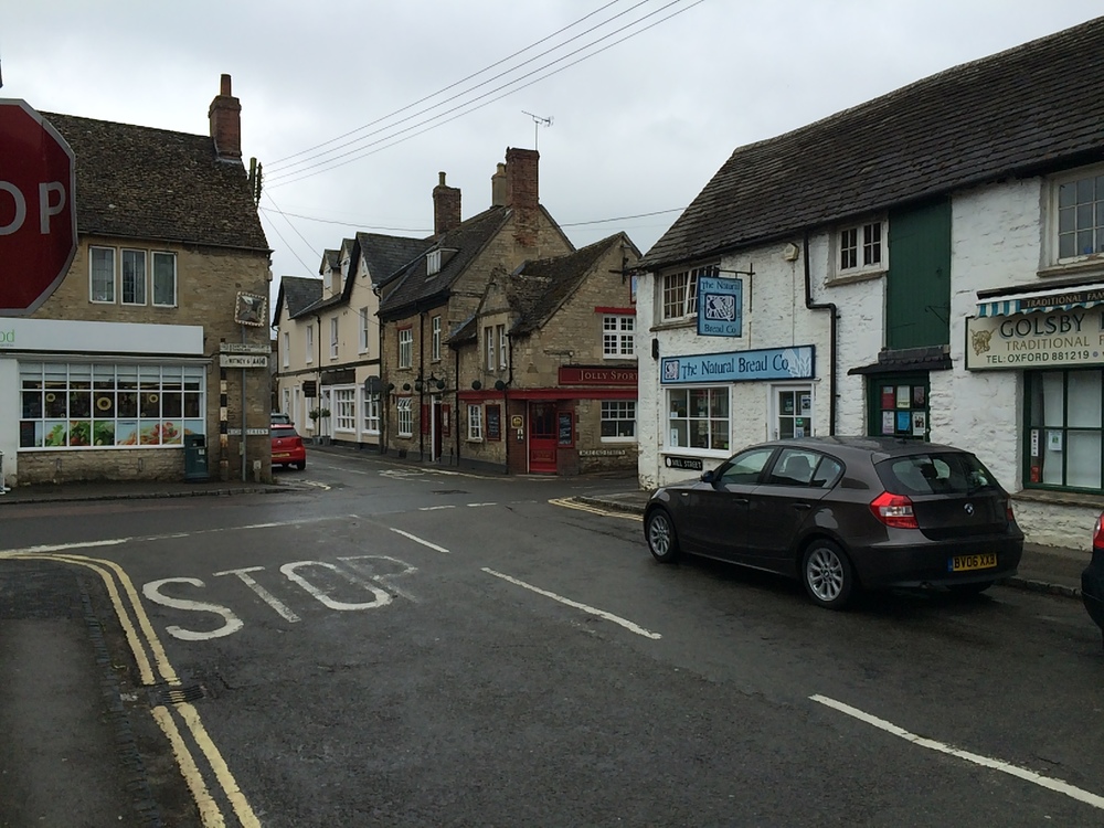
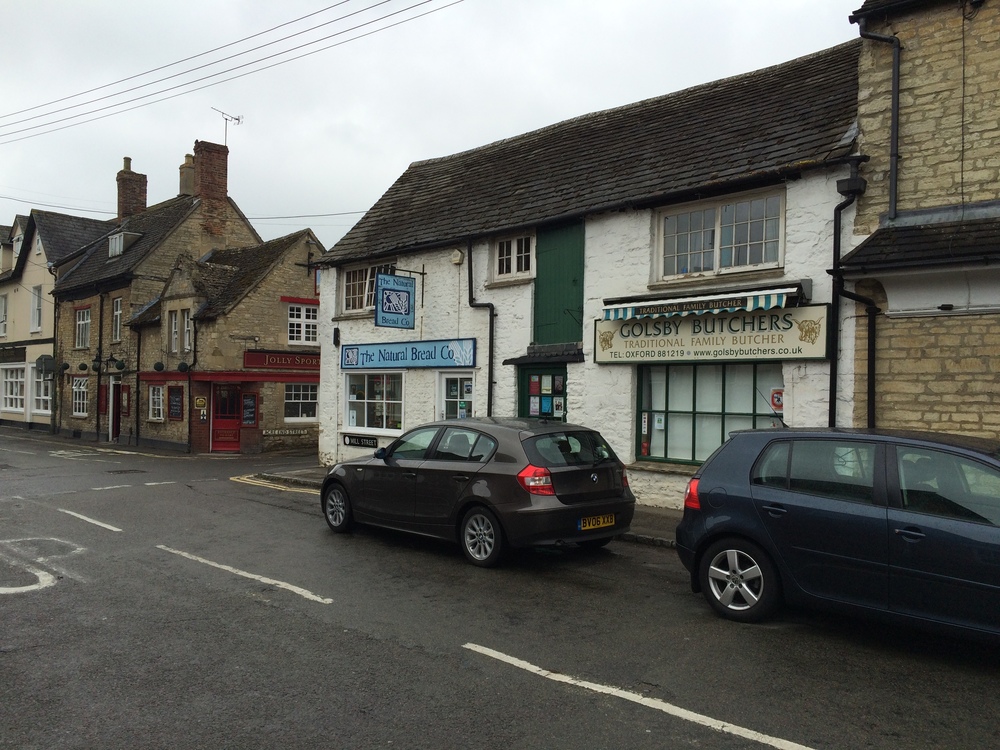
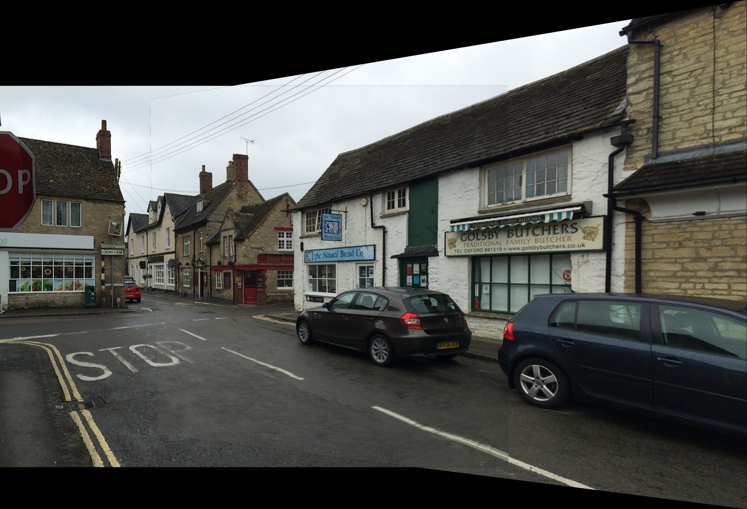
Recall from the introduction that a keypoint has a location \(\pB_i\) and descriptor \(\dB_i\). There are many types of keypoints used. Traditionally this course has used SIFT and SURF, but these are subject to patents and installed in only a few versions of opencv. Traditionally, this has led to homework 3 being an exercise in figuring out how to install a very special version of opencv (and then figuring out some undocumented features).

We provide another descriptor called AKAZE (plus some other features) in common.py. In addition to this descriptor, you are encouraged to look at common.py to see if there are things you want to use while working on the homework.

The calling convention is: keypoints, descriptors = common.get_AKAZE(image) which will give you a \(N \times 4\) matrix keypoints and a \(N \times F\) matrix descriptors containing descriptors for each keypoint. The first two columns of keypoints contain \(x,y\); the last two are the angle and (roughly) the scale at which they were found in case those are of interest. The descriptor has also been post-processed into something where \(\|\dB_i - \dB_j'\|^2_2\) is meaningful.

Files: We provide you with a number of panoramas in task6/ that you can choose to merge together. To enable you to run your code automatically on multiple panoramas without manually editing filenames (see also os.listdir), we provide them in a set of folders.

Each folder contains two images: (a) p1.jpg; and (b) p2.jpg. Some also contain images (e.g., p3.jpg) which may or may not work. You should be able to match all the provided panoramas; you should be able to stitch all except for florence3 and florence3_alt.

(3 points) Fill in compute_distance in task6.py. This should compute the pairwise squared L2 distance between two matrices of descriptors. You can and should use the \(\|\xB-\yB\|^2_2 = \|\xB\|^2_2 + \|\yB\|^2_2 - 2 \xB^T \yB\) trick from HW0, numpy test 11.
(5 points) Fill in find_matches in task6.py. This should use compute_distance plus the ratio test from the foreword to return the matches. You will have to pick a threshold for the ratio test. Something between \(0.7\) and \(1\) is reasonable, but you should experiment with it (look output of the draw_matches once you complete it).

Beware! The numbers for the ratio shown in the lecture slides apply to SIFT; the descriptor here is different so the ratio threshold you should use is different.

Look at np.argsort as well as np.take_along_axis.
(5 points) Fill in draw_matches in task6.py. This should put the images on top of each other and draw lines between the matches. You can use this to debug things.

Use cv2.line.
(3 points) Put a picture of the matches between two image pairs of your choice in your report.
(10 points) Fill in RANSAC_fit_homography in homography.py.

This should RANSACify fit_homography. You should keep track of the best set of inliers you have seen in the RANSAC loop. Once the loop is done, please re-fit the model to these inliers. In other words, if you are told to run \(N\) iterations of RANSAC, you should fit a homography \(N\) times on the minimum number of points needed; this should be followed by a single fitting of a homography on many more points (the inliers for the best of the \(N\) models). You will need to set epsilon’s default value: \(0.1\) pixels is too small; \(100\) pixels is too big. You will need to play with this to get the later parts to work.

When sampling correspondences, draw without replacement; if you do it with replacement you may pick the same point repeatedly and then try to (effectively) fit a model to three points.
(18 points) Fill in make_warped and warp_and_combine in task6.py. This should take two images as an argument and do the whole pipeline described in the foreword. The resulting image should use cv2.warpPerspective to make a merged image where both images fit in. This merged image should have: (a) image 1’s pixel data if only image 1 is present at that location; (b) image 2’s pixel data if only image 2 is present at that location; (c) the average of image 1’s data and image 2’s data if both are present. You can do so by using a warped mask.

*Walkthrough of warp_and_combine *:
1. There is an information bottleneck in estimating \(\HB\). If \(\HB\) is correct, then you’re set; if it’s wrong, there’s nothing you can do. First make sure your code estimates \(\HB\) right.
2. Pick which image you’re going to merge to; without loss of generality, pick image 1. Figure out how to make a merged image that’s big enough to hold both image 1 and transformed image 2. Think of this as finding the smallest enclosing rectangle of both images. The merged image should be bigger than all input image in size. The upper left corner of this rectangle (i.e., pixel \([0,0]\)) may not be at the same location as in image 1. You will almost certainly need to hand-make a homography that translates image 1 to its location in the merged image. For doing this calculations, use the fact that the image content will be bounded by the image corners. Looking at the min, max of these gives you what you need to create the panorama.
3. Warp both images to the merged image. You can figure out where the images go by warping images containing ones to the merged images instead of the image and filling the image with 0s where the image doesn’t go. These masks also tell you how to create the average.
4. Be careful about your order of applying the homography. Think about are you warping image2 into image1’s perspective or the other way around. If you want to reverse the homography effect, you can just inverse the homography matrix.
Debugging Hints:
- Make a fake pair of images by taking an image, rolling it by \((10,30)\) and then saving it. Debugging this is far easier if you know what the answer should be.
- If you want to debug the warping, you can also provide two images that are crops of the same image, (e.g., I[100:400,100:400] and I[150:450,75:375]) where you know the homography (since it is just a translation).
(3 points) Put merges from two of your favorite pairs in the report. You can either choose an image we provide you or use a pair of images you take yourself.
(3 points) Put these merges as mypanorama1.jpg and mypanorama2.jpg in your zip submission.

Augmented Reality on a Budget

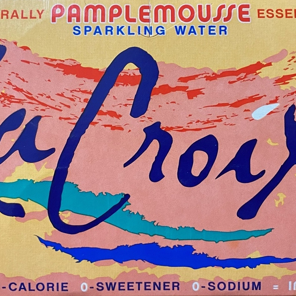
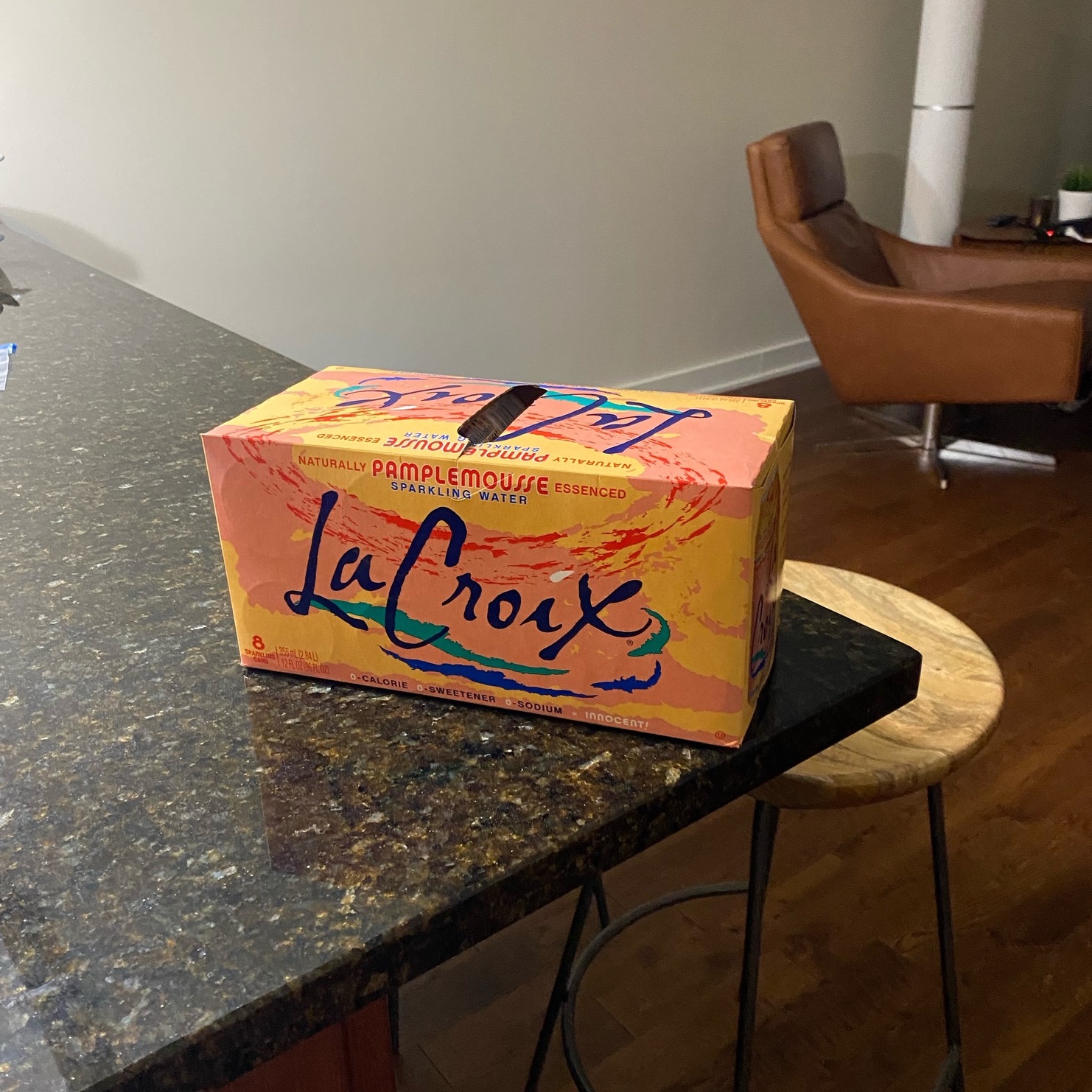
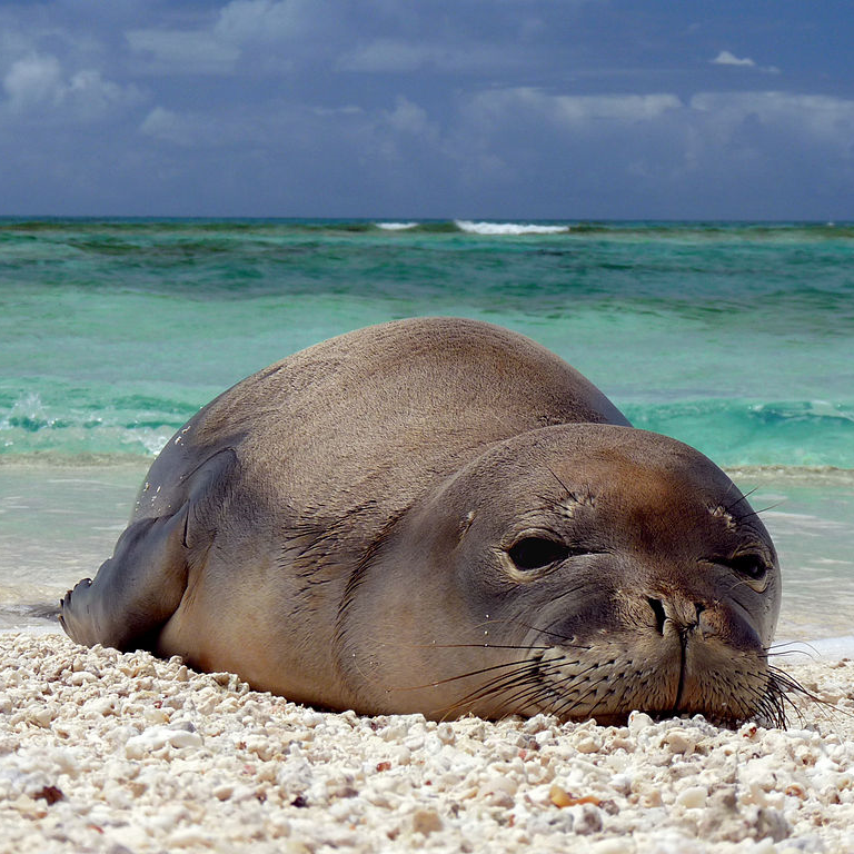
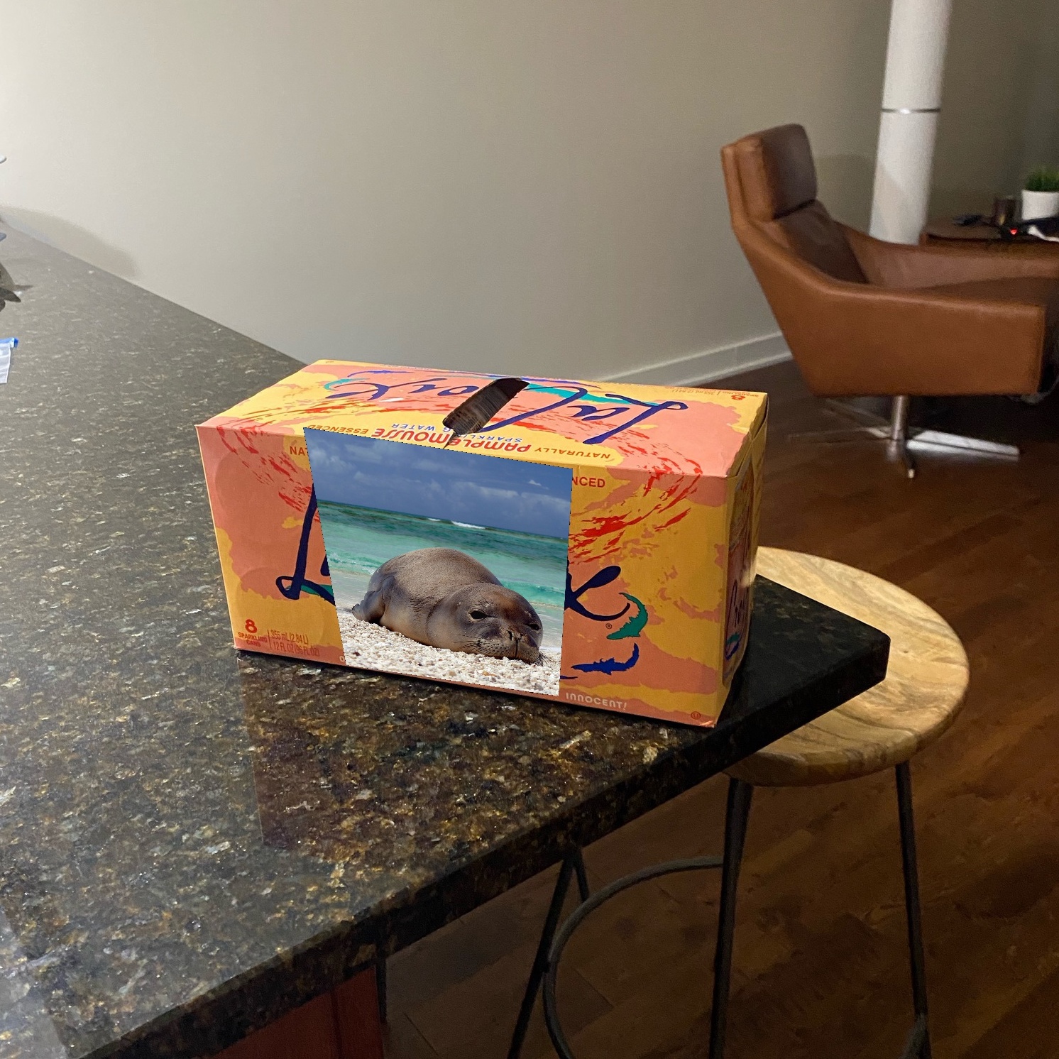
Task 7: Augmented Reality on a Budget

If you can warp images together, you can replace things in your reality. Imagine that we have a template image and this template appears in the world but viewed at an angle. You can fit a homography mapping between the template and the scene. Once you have a homography, you can transfer anything. This enables you to improve things.

Files: We give a few examples of templates and scenes in task7/scenes/. Each folder contains: template.png: a viewed-from-head-on / distortion-free / fronto-parallel version of the texture; and scene.jpg: an image where the texture appears at some location and viewed at some angle. We provide a set of seals (e.g., the UM seal) that you may want to put on things in task7/seals/. You can substitute whatever you like.

(3 points) Fill in the function improve_image(scene,template,transfer) in task7.py that aligns template to scene using a homography, just as in task 6. Then, instead of warping template to the image, warp transfer. If you want to copy over your functions from task 6, you can either import them or just copy them.
- The matches that you get are definitely not one-to-one. You’ll probably get better results if you match from the template to the scene (i.e., for each template keypoint, find the best match in scene). Be careful about ordering though if you transfer your code!
- The image to transfer might not be the same size as the template. You can either resize transfer to be the same size as template or automatically generate a homography.
- For using the fucntion warp_and_combine from task 6, you may want to change it a little bit, since you should make sure you use warped template to cover areas in the scene completely as shown in Figure 3.
(2 points) Do something fun with this. Submit a synthetically done warp of something interesting. If you do something particularly neat to get the system to work, please write this in the report.

Include the images in your report. In addition, submit in your zip file the following files:
- myscene.jpg – the scene
- mytemplate.png OR mytemplate.jpg – the template. Submit either png or jpg but not both.
- mytransfer.jpg – the thing you transfer
- myimproved.jpg – your result
Guidelines: If you try this on your own images, here are some suggestions:
- Above all, please be respectful.
- This sort of trick works best with something that has lots of texture across the entire template. The lacroix carton works very well. The aep.jpg image that you saw in dithering does not work so well since it has little texture for the little building at the bottom.
- This trick is most impressive if you do this for something seen at a very different angle. You may be able to extend how far you can match by pre-generating synthetic warps of the template (i.e, generate \(\textrm{synth}_i = \textrm{apply}(\HB_i,T)\) for a series of \(\HB_i\), then see if you can find a good warping \(\hat{\HB}\) from \(\textrm{synth}_i\) to the scene. Then the final homography is \(\hat{\HB} \HB_i\).

Tasks Checklist

This section is meant to help you keep track of the many things that go in the report:

Canvas Submission Checklist

In the zip file you submit to Canvas, the directory named after your uniqname should include the following files:

common.py – do not edit though; this may be substituted
homography.py
task5.py
task6.py
mypanorama1.jpg, mypanorama2.jpg
task7.py
myscene.jpg, mytemplate.png/jpg, mytransfer.jpg, myimproved.jpg

The following are optional:

myfavoritepanorama.jpg