EECS 442: Computer Vision (Winter 2024)
Homework 4 – Machine Learning
Instructions
This homework is due at 11:59 p.m. on Wednesday March 20th, 2024.
This homework is divided into two major sections based on how you’re expected to write code:
Section 1:
- You’ll be writing the code in the same way you’ve been doing until now, i.e., in simple python files.
Section 2:
- We are going to use Google Colab or local Jupyter Notebook on your on machine (both GPU and CPU) to run our code. For more information on using Colab, please see the official Colab tutorial. The whole assignment is designed to be CPU friendly, but we still strongly encourage you try with Colab first.
- We have also provided you with the python file version of the assignment in
python_backupfolder, but since the assignment is originally designed for Jupyter Notebook only, we strongly suggest you do this assignment in Jupyter Notebook. This option is provided only to backup the case of Colab failure or local Jupyter Notebook problem. If you’re doing the homework in the python files, please attach your terminal output to the report. - To do the homework on Colab, you just need to login to Colab with your Google/UMich account and upload corresponding notebook to the Colab (
File -> Upload notebook), then you can get started.
The submission includes two parts:
-
To Canvas: submit a
zipfile containing a single directory with your uniqname as the name that contains all your code and anything else asked for on the Canvas Submission Checklist. Don’t add unnecessary files or directories. Starter code is given to you on Canvas under the “Homework 4” assignment. You can also download it here. Clean up your submission to include only the necessary files. Pay close attention to filenames for autograding purposes.- We have indicated questions where you have to do something in code in red. If Gradescope asks for it, also submit your code in the report with the formatting below.
Submission Tip: Use the Tasks Checklist and Canvas Submission Checklist at the end of this homework. We also provide a script that validates the submission format here.
-
To Gradescope: submit a
pdffile as your write-up, including your answers to all the questions and key choices you made.- We have indicated questions where you have to do something in the report in green. Coding questions also need to be included in the report.
You might like to combine several files to make a submission. Here is an example online link for combining multiple PDF files. The write-up must be an electronic version. No handwriting, including plotting questions. \(\LaTeX\) is recommended but not mandatory.
For including code, do not use screenshots. Generate a PDF using a tool like this or using this Overleaf LaTeX template. If this PDF contains only code, be sure to append it to the end of your report and match the questions carefully on Gradescope.
For
.ipynbnotebooks in your local system you may refer to this post to convert your notebook to a pdf usingnbconvert. For Google-Colab users, you may use this code snippet as the final cell to download your notebooks as pdf’s.# generate pdf # 1. Find the path to your notebook in your google drive. # 2. Please provide the full path of the notebook file below. # Important: make sure that your file name does not contain spaces! # Syntax: # notebookpath = '/content/drive/MyDrive/HW4/notebook.ipynb' # import os from google.colab import drive from google.colab import files drive_mount_point = '/content/drive/' drive.mount(drive_mount_point) notebookpath = '<notebook_path>' file_name = notebookpath.split('/')[-1] get_ipython().system("apt update && apt install texlive-xetex texlive-fonts-recommended texlive-generic-recommended") get_ipython().system("jupyter nbconvert --to PDF {}".format(notebookpath.replace(' ', '\\ '))) files.download(notebookpath.split('.')[0]+'.pdf') # PDF will be downloaded in the same directory as the notebook, with the same name.
Python Environment
To make your life easier, we recommend you to install the latest Anaconda for Python 3.7. This is a Python package manager that includes most of the modules you need for this course. We will make use of the following packages extensively in this course:
Local Development
If you’re doing this homework on your local machine instead of Colab, then other than the packages you should have already installed in previous homework, you will also need: tqdm, pytorch>=1.8.0, torchvision and torchsummary of the corresponding version. You may install these packages using anaconda or pip. Notice that some of the packages may need to be downloaded from certain anaconda channel, you may need to search on the Anaconda official website for more instructions.
Section 1
Computational Graphs and Backprop
We have seen that representing mathematical expressions as computational graphs allows us to easily compute gradients using backpropagation. After writing a mathematical expression as a computational graph, we can easily translate it into code. In this problem you’ll gain some experience with backpropagation in a simplified setting where all of the inputs, outputs, and intermediate values are all scalar values instead vectors, matrices, or tensors.
In the forward pass we receive the inputs (leaf nodes) of the graph and compute the output. The output is typically a scalar value representing the loss \(L\) on a minibatch of training data.
In the backward pass we compute the derivative of the graph’s output \(L\) with respect to each input of the graph. There is no need to reason globally about the derivative of the expression represented by the graph; instead when using backpropagation we need only think locally about how derivatives flow backward through each node of the graph. Specifically, during backpropagation a node that computes \(y=f(x_1, \ldots, x_N)\) receive an upstream gradient \(\pd{L}{y}\) giving the derivative of the loss with respect the the node output and computes downstream gradients \(\pd{L}{x_1},\ldots,\pd{L}{x_N}\) giving the derivative of the loss with respect to the node inputs.
Here’s an example of a simple computational graph and the corresponding code for the forward and backward passes. Notice how each outgoing edge from an operator gives rise to one line of code in the forward pass, and each ingoing edge to an operator gives rise to one line of code in the backward pass.
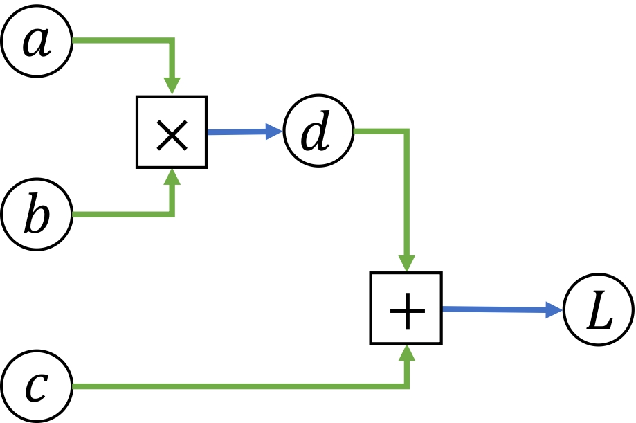
def f(a, b, c):
	d = a * b       # Start forward pass
	L = c + d

	grad_L = 1.0    # Start backward pass
	grad_c = grad_L
	grad_d = grad_L
	grad_a = grad_d * b
	grad_b = grad_d * a

	return L, (grad_a, grad_b, grad_c)
Sometimes you’ll see computational graphs where one piece of data is used as input to multiple operations. In such cases you can make the logic in the backward pass cleaner by rewriting the graph to include an explicit copy operator that returns multiple copies of its input. In the backward pass you can then compute separate gradients for the two copies, which will sum when backpropagating through the copy operator:
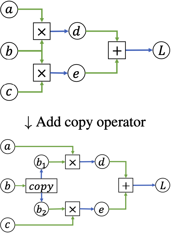
def f(a, b, c):
	# Start forward pass
	b1 = b
	b2 = b
	d = a * b1
	e = c * b2
	L = d + e

	# Start backward pass
	grad_L = 1.0
	grad_d = grad_L
	grad_e = grad_L
	grad_a = grad_d * b1
	grad_b1 = grad_d * a
	grad_c = grad_e * b2
	grad_b2 = grad_e * c
	# Sum grads for copies
	grad_b = grad_b1 + grad_b2

	return L, (grad_a, grad_b, grad_c)
Task 1: Implementing Computational Graphs
Below we’ve drawn three computational graphs for you to practice implementing forward and backward passes. The functions f1 and f2 are optional, and the function f3 is required. The file backprop/functions.py contains stubs for each of these computational graphs. You can use the driver program backprop/backprop.py to check your implementation.
- (10 points) Implement the forward and backward passes for the computational graph
f3below.
The file backprop/backprop-data.pkl contains sample inputs and outputs for the three computational graphs; the driver program loads inputs from this file for you when checking your forward passes.
To check the backward passes, the driver program implements numeric gradient checking. Given a function \(f:\RR\to\RR\), we can approximate the gradient of \(f\) at a point \(x_0\in\RR\) as:
\[\pd{f}{x}(x_0) \approx \frac{f(x_0 + h) - f(x_0 - h)}{2h}\]Each of these computational graphs implements a function or operation commonly used in machine learning. Can you guess what they are? (This is just for fun, not required).
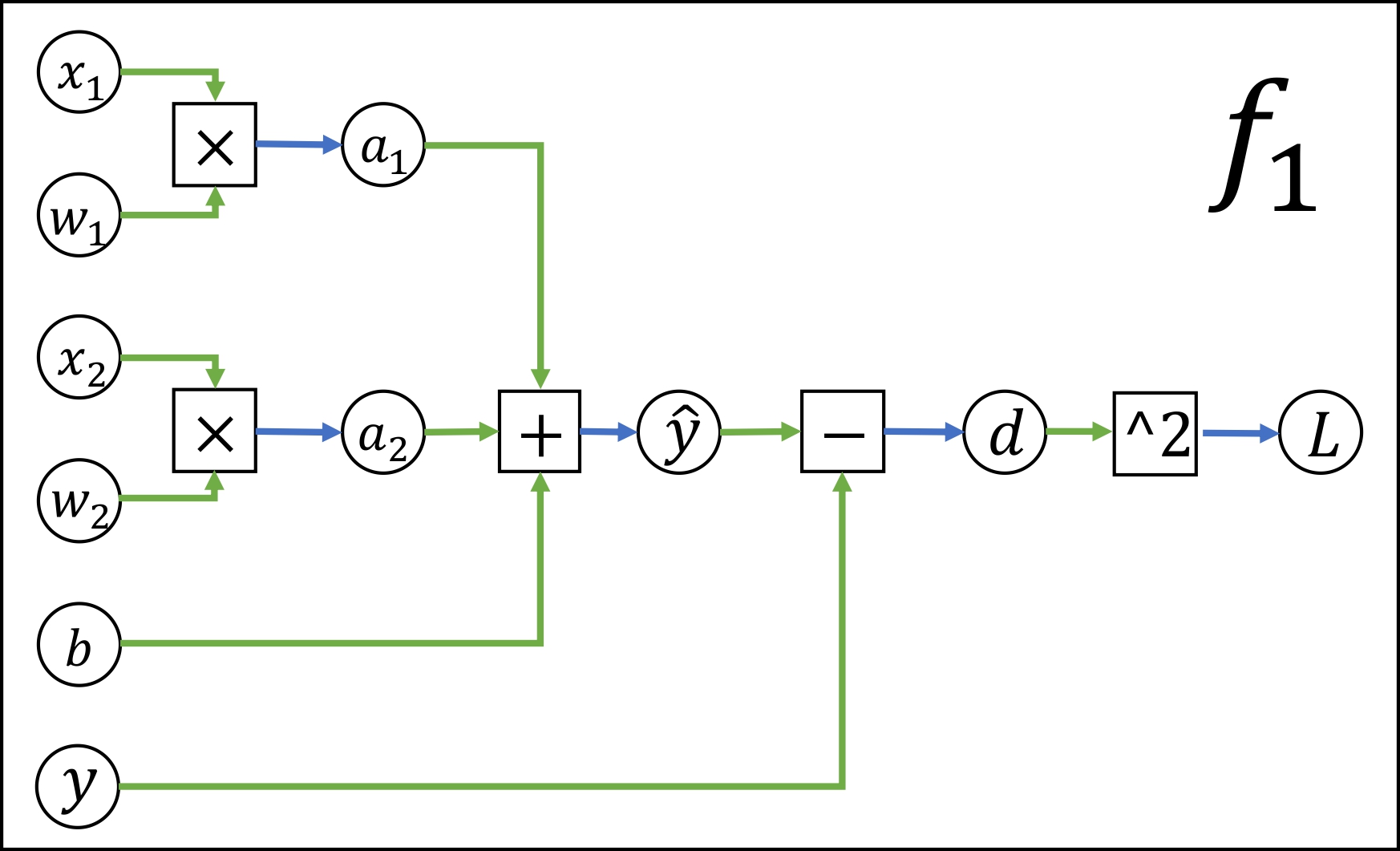
f1 (optional)
The subtraction node computes \(d = \hat y - y\)
The ^2 node computes \(L = d^2\)

f2: (optional)
The \(\times2\) node computes \(d = 2x\)
The \(\div\) node computes \(y = t / b\)
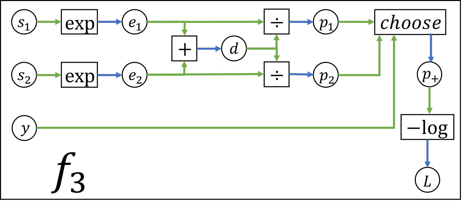
f3: (required - 10 points)
\(y\) is an integer equal to either 1 or 2. You don’t need to compute a gradient for \(y\).
The \(\div\) nodes compute \(p_1 = e_1 / d\) and \(p_2 = e_2 / d\).
The choose node outputs outputs \(p_1\) if \(y=1\), and outputs \(p_2\) if \(y=2\).
Write Your Own Graph (Optional)
In your report, draw a computational graph for any function of your choosing. It should have at least five operators. (You can hand-draw the graph and include a picture of it in your report.)
In the file backprop/functions.py, implement a forward and backward pass through your computational graph in the function f4. You can modify the function to take any number of input arguments. After implementing f4, you can use the driver script to perform numeric gradient checking. Depending on the functions in your graph, you may see errors \(\geq10^{-8}\) even with a correct backward pass. This is ok!
Fully-Connected Neural Networks
In this question you will implement and train a fully-connected neural network to classify images.
For this question you cannot use any deep learning libraries such as PyTorch or TensorFlow.
Task 2: Modular Backprop API
In the previous questions on this assignment you used backpropagation to compute gradients by implementing monolithic functions that combine the forward and backward passes for an entire graph. As we’ve discussed in lecture, this monolithic approach to backpropagation isn’t very modular – if you want to change some component of your graph (new loss function, different activation function, etc) then you need to write a new function from scratch.
Rather than using monolithic backpropagation implementations, most modern deep learning frameworks use a modular API for backpropagation. Each primitive operator that will be used in a computational graph implements a forward function that computes the operator’s output from its inputs, and a backward function that receives upstream gradients and computes downstream gradients. Deep learning libraries like PyTorch or TensorFlow provide many predefined operators with corresponding forward and backward functions.
To gain experience with this modular approach to backpropagation, you will implement your own miniature modular deep learning framework. The file neuralnet/layers.py defines forward and backward functions for several common operators that we’ll need to implement our own neural networks.
Each forward function receives one or more numpy arrays as input, and returns:
- A numpy array giving the output of the operator;
- A cache object containing values that will be needed during the backward pass. The backward function receives a numpy array of upstream gradients along with the cache object, and must compute and return downstream gradients for each of the inputs passed to the forward function.
Along with forward and backward functions for operators to be used in the middle of a computational graph, we also define functions for loss functions that will be used to compute the final output from a graph. These loss functions receive an input and return both the loss and the gradient of the loss with respect to the input.
This modular API allows us to implement our operators and loss functions once, and reuse them in different computational graphs. For example, we can implement a full forward and backward pass to compute the loss and gradients for linear regression in just a few lines of code:
from layers import fc_forward, fc_backward, l2_loss

def linear_regression_step(X, y, W, b):
    y_pred, cache = fc_forward(X, W, b)
    loss, grad_y_pred = l2_loss(y_pred, y)
    grad_X, grad_W, grad_b = fc_backward(grad_y_pred, cache)
    return grad_W, grad_b
In the file neuralnet/layers.py you need to complete the implementation of the following:
-
(5 points) Fully-connected layer:
fc_forwardandfc_backward. -
(5 points) ReLU nonlinearity:
relu_forwardandrelu_backwardwhich applies the function \(ReLU(x_i) = \max(0, x)\) elementwise to its input. -
(5 points) Softmax Loss Function:
softmax_loss.The softmax loss function receives a matrix \(x\in\RR^{N\times C}\) giving a batch of classification scores for \(N\) elements, where for each element we have a score for each of \(C\) different categories. The softmax loss function first converts the scores into a set of \(N\) probability distributions over the elements, defined as:
\[p_{i,c} = \cfrac{\exp(x_{i,c})}{\sum_{j=1}^C \exp(x_{i,j})}\]The output of the softmax loss is then given by:
\[L = -\frac{1}{N} \sum_{i=1}^N \log(p_{i,y_i})\]where \(y_i\in\{1,\ldots,C\}\) is the ground-truth label for the \(i\)th element.
A naive implementation of the softmax loss can suffer from numeric instability. More specifically, large values in \(x\) can cause overflow when computing \(\exp\). To avoid this, we can instead compute the softmax probabilities as:
\[p_{i,c} = \frac{\exp(x_{i,c} - M_i)}{\sum_{j=1}^C \exp(x_{i,j} - M_i)}\]where \(M_i = \max_c x_{i,c}\).
This ensures that all values we exponentiate are \(<0\), avoiding any potential overflow. It’s not hard to see that these two formulations are equivalent, since
\[\frac{\exp(x_{i,c} - M_i)}{\sum_{j=1}^C\exp(x_{i,j} - M_i)} = \frac{\exp(x_{i,c})\exp(-M_i)}{\sum_{j=1}^C \exp(x_{i,j})\exp(-M_i)} = \frac{\exp(x_{i,c})}{\sum_{i=1}^C \exp(x_{i,j})}\]Your softmax implementation should use this max-subtraction trick for numeric stability. You can run the script
neuralnet/check_softmax_stability.pyto check the numeric stability of your softmax loss implementation.Your implementation of
softmax_lossshould return the loss value and the gradients. For detailed information about gradients of softmax-loss function, refer these notes. -
(5 points) L2 Regularization:
\[L(W) = \frac{\lambda}{2}\|W\|^2 = \frac{\lambda}{2} \sum_i W_i^2\]l2_regularizationwhich implements the L2 regularization losswhere the sum ranges over all scalar elements of the weight matrix \(W\) and \(\lambda\) is a hyperparameter controlling the regularization strength.
After implementing all functions above, you can use the script neuralnet/gradcheck_layers.py to perform numeric gradient checking on your implementations. The difference between all numeric and analytic gradients should be less than \(10^{-9}\).
Keep in mind that numeric gradient checking does not check whether you’ve correctly implemented the forward pass; it only checks whether the backward pass you’ve implemented actually computes the gradient of the forward pass that you implemented.
Task 3: Implement a Two-Layer Network
Your next task is to implement a two-layer fully-connected neural network using the modular forward and backward functions that you just implemented.
In addition to using a modular API for individual layers, we will also adopt a modular API for classification models as well. This will allow us to implement multiple different types of image classification models, but train and test them all with the same training logic.
The file neuralnet/classifier.py defines a base class for image classification models. You don’t need to implement anything in this file, but you should read through it to familiarize yourself with the API. In order to define your own type of image classification model, you’ll need to define a subclass of Classifier that implements the parameters, forward, and backward methods.
In the file neuralnet/linear_classifier.py we’ve implemented a LinearClassifier class that subclasses Classifier and implements a linear classification model using the modular layer API from the previous task together with the modular classifier API. Again, you don’t need to implement anything in this file but you should read through it to get a sense for how to implement your own classifiers.
Now it’s your turn! In the file neuralnet/two_layer_net.py we’ve provided the start to an implementation of a TwoLayerNet class that implements a two-layer neural network (with ReLU nonlinearity).
- (10 points) Complete the implementation of the
TwoLayerNetclass. Your implementations for theforwardandbackwardmethods should use the modular forward and backward functions that you implemented in the previous task.
After completing your implementation, you can run the script gradcheck_classifier.py to perform numeric gradient checking on both the linear classifier we’ve implemented for you as well as the two-layer network you’ve just implemented. You should see errors less than \(10^{-10}\) for the gradients of all parameters.
Task 4: Training Two-Layer Networks
You will train a two-layer network to perform image classification on the CIFAR-10 dataset. This dataset consists of \(32\times 32\) RGB images of 10 different categories. It provides 50,000 training images and 10,000 test images. Here are a few example images from the dataset:
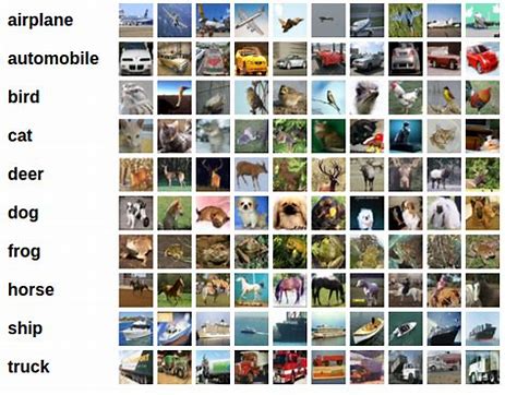
You can use the script neuralnet/download_cifar.sh to download and unpack the CIFAR10 dataset.
The file neuralnet/train.py implements a training loop.
We’ve already implemented a lot of the logic here for you.
You don’t need to do anything with the following files, but you can look through them to see how
they work:
neuralnet/data.pyprovides a function to load and preprocess the CIFAR10 dataset, as well as aDataSamplerobject for iterating over the dataset in minibatches.neuralnet/optim.pydefines anOptimizerinterface for objects that implement optimization algorithms, and implements a subclassSGDwhich implements basic stochastic gradient descent with a constant learning rate.
-
Implement the
training_stepfunction in the fileneuralnet/train.py.This function inputs the model, a minibatch of data, and the regularization strength; it computes a forward and backward pass through the model and returns both the loss and the gradient of the loss with respect to the model parameters. The loss should be the sum of two terms:
- A data loss term, which is the softmax loss between the model’s predicted scores and the ground-truth image labels
- A regularization loss term, which penalizes the L2 norm of the weight matrices of all the fully-connected layers of the model. You should not apply L2 regularization to the biases.
Now it’s time to train your model! Run the script neuralnet/train.py to train a two-layer network on the CIFAR-10 dataset. The script will print out training losses and train and val set accuracies as it trains. After training concludes, the script will also mke a plot of the training losses as well as the training and validation-set accuracies of the model during training; by default this will be saved in a file plot.pdf, but this can be customized with the flag --plot-file. You should see a plot that looks like this:
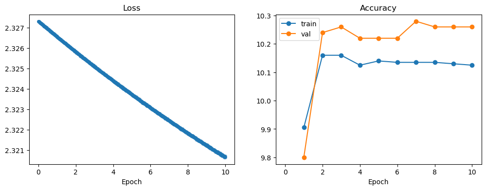
Unfortunately, it seems that your model is not training very effectively – the training loss has not decreased much from its initial value of \(\approx2.3\), and the training and validation accuracies are very close to \(10\%\) which is what we would expect from a model that randomly guesses a category label for each input.
You will need to tune the hyperparameters of your model in order to improve it. Try changing the hyperparameters of the model in the provided space of the main function of neuralnet/train.py. You can consider changing any of the following hyperparameters:
num_train: The number of images to use for traininghidden_dim: The width of the hidden layer of the modelbatch_size: The number of examples to use in each minibatch during SGDnum_epochs: How long to train the model. An epoch is a single pass through the training set.learning_rate: The learning rate to use for SGDreg: The strength of the L2 regularization term
You should tune the hyperparameters and train a model that achieves at least \(40\%\) on the validation set. After tuning your model, run your best model exactly once on the test set using the script neuralnet/test.py.
-
In your report, include the loss / accuracy plot for your best model, describe the hyperparameter settings you used, and give the final test-set performance of your model.
You may not need to change all of the hyperparameters; some are fine at their default values. Your model shouldn’t take an excessive amount of time to train. For reference, our hyperparameter settings achieve \(\approx45\%\) accuracy on the validation set in \(\approx5\) minutes of training on a 2019 MacBook Pro.
To gain more experience with hyperparameters, you should also tune the hyperparameters to find a setting that results in an overfit model that achieves \(\geq75\%\) accuracy on the training set.
-
In your report, include the loss / accuracy plot for your overfit model and describe the hyperparameter settings you used.
As above, this should not take an excessive amount of training time – we are able to train an overfit model that achieves \(\approx80\%\) accuracy on the training set within about a minute of training.
It’s easier to overfit a smaller training set.
Section 2
Fashion-MNIST Classification
In this part, you will implement and train Convolutional Neural Networks (ConvNets) in PyTorch to classify images. Unlike previous section, backpropagation is automatically inferred by PyTorch in this assignment, so you only need to write code for the forward pass. If you still not familiar with the auto gradient feature of the PyTorch, we strongly encourage you to go through the official tutorial for TORCH.AUTOGRAD.
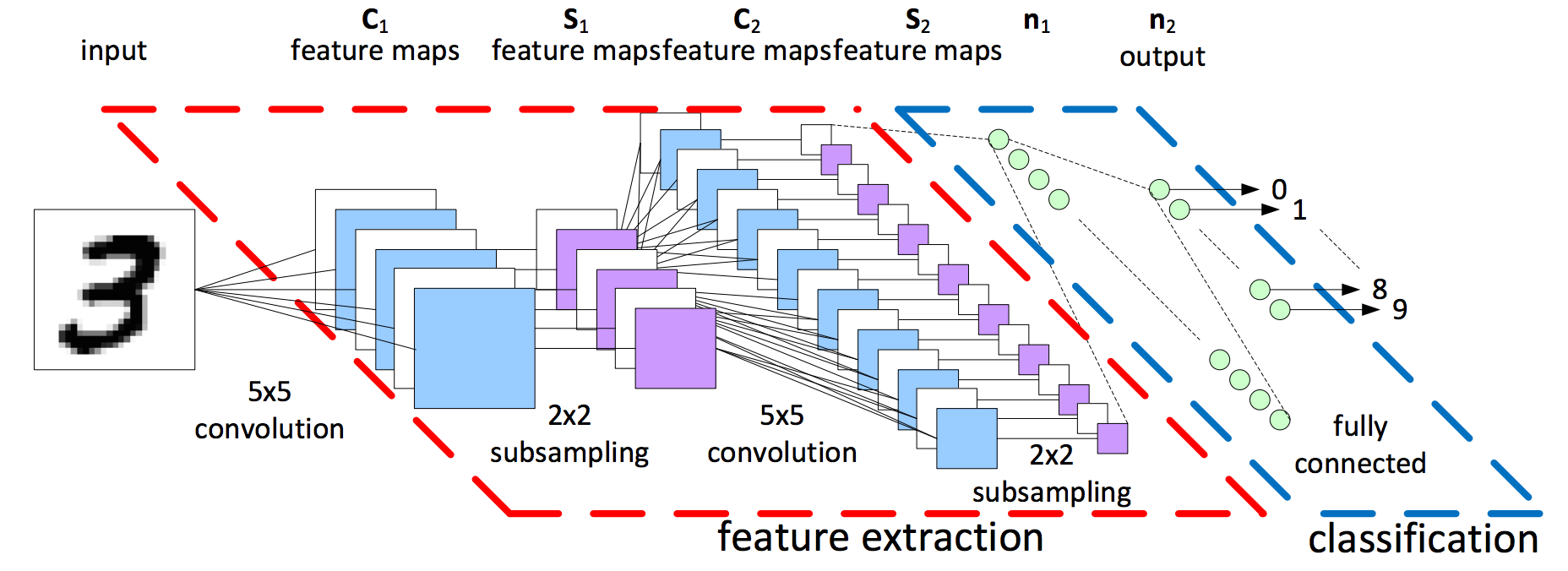
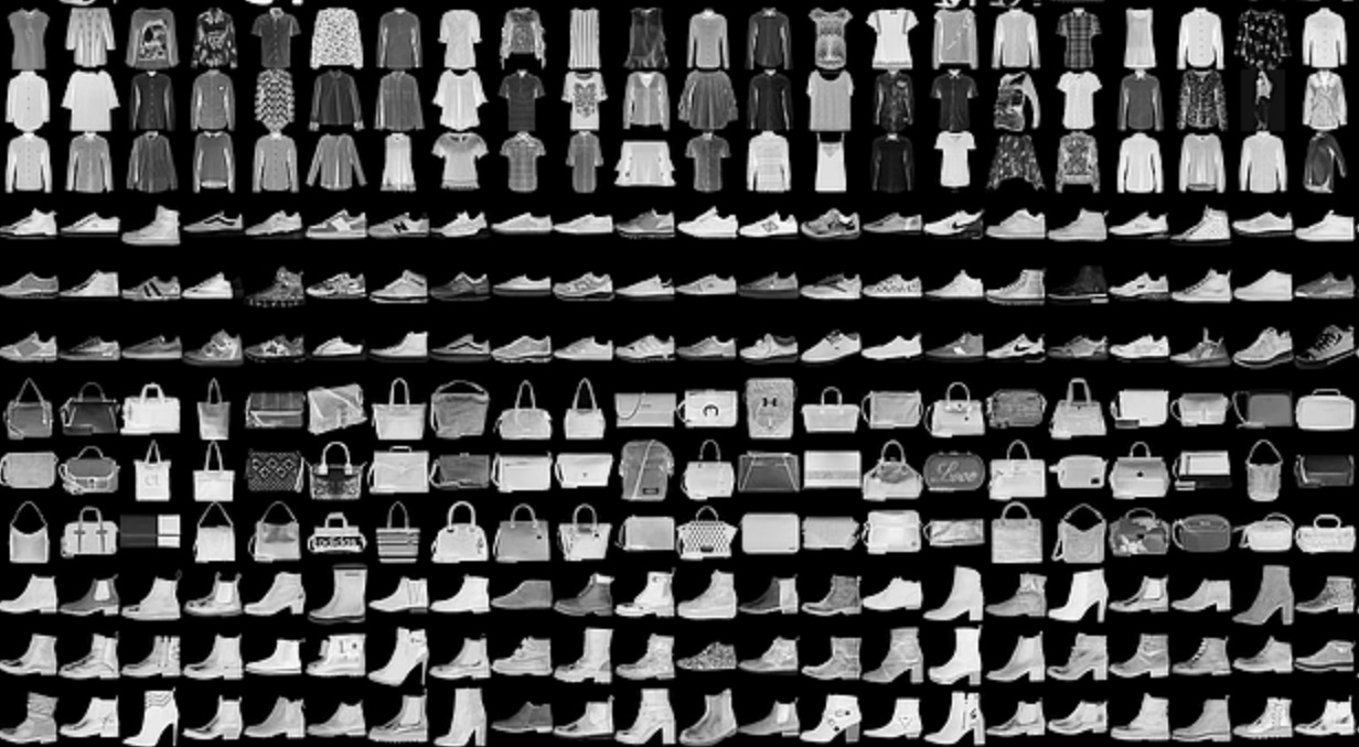
The dataset we use is the Fashion-MNIST dataset, which is available here and in torchvision.datasets. Fashion-MNIST has 10 classes, 60000 training+validation images (we have split it to have 50000 training images and 10000 validation images, but you can change the numbers), and 10000 test images.
Task 5: Train Your Own Classification Model
Open the part1.ipynb notebook in Google Colab/local Jupyter Notebook and implement the following:
- The architecture of the network (define layers and implement forward pass)
- The optimizer (SGD, RMSProp, Adam, etc.) and its parameters. (
weight_decayis the L2 regularization strength) - Training parameters (batch size and number of epochs)
You should train your network on training set and change those hyperparameters listed above based on evaluation on the validation set. You should run evalution on the test set only once at the end.
Complete the following:
- (15 points) Submit the notebook (with outputs) that trains with your best combination of model architecture, optimizer and training parameters, and evaluates on the test set to report an accuracy at the end.
- (10 points) Report the detailed architecture of your best model. Include information on hyperparameters chosen for training and a plot showing both training and validation accuracy across iterations.
- (5 points) Report the accuracy of your best model on the test set. We expect you to achieve over 85%.
Read PyTorch documentation for torch.nn and pick layers for your network. Some common choices are:
nn.Linearnn.Conv2d, try different number of filters (out_channels) and size of filters (kernel_size)nn.ReLU, which provides non-linearity between layersnn.MaxPool2dandnn.AvgPool2d, two kinds of pooling layernn.Dropout, which helps reduce overfitting
Your network does not need to be complicated. We achieved over 85% test accuracy with two convolutional layers, and it took less than 5 mins to train on Colab and less than 10 mins on local CPU machine. You will get partial credits for any accuracy over 70%, so do not worry too much and spend your time wisely.
Task 6: Pre-trained NN
In order to get a better sense of the classification decisions made by convolutional networks, your job is now to experiment by running whatever images you want through a model pretrained on ImageNet.
These can be images from your own photo collection, from the internet, or somewhere else but they should belong to one of the ImageNet classes. Look at the idx2label dictionary in part2.ipynb for all the ImageNet classes.
For this task, you have to find:
- One image (
img1) where the pretrained model gives reasonable predictions, and produces a category label that seems to correctly describe the content of the image - One image (
img2) where the pretrained model gives unreasonable predictions, and produces a category label that does not correctly describe the content of the image.
You can upload images in Colab by using the upload button on the top left. For more details on how to upload files on Colab, please see our Colab tutorial. For local Jupyter Notebook users, you may simply put the image under the same folder with the notebook and open it as you will do in a normal python file.
- (10 points) Submit the two images with their predicted classes in your report, we have provided you with the code to generate this image in the notebook.
Tasks Checklist
This section is meant to help you keep track of the many things that go in the report:
- Implementing Computational Graphs:
- 1.1 -
f3(required);f1andf2(optional) - 1.2 - (optional) Draw a computational graph and implement forward/backward
- 1.1 -
- Modular Backprop API:
- 2.1 -
fc_forwardandfc_backward - 2.2 -
relu_forwardandrelu_backward - 2.3 -
softmax_loss - 2.4 -
l2_regularization
- 2.1 -
- Implement Two-Layer Network:
- 3.1 -
TwoLayerNet
- 3.1 -
- Train Two-Layer Network:
- 4.1 -
training_step - 4.2 - Results of best model
- 4.3 - Results of overfit model
- 4.1 -
- Train Your Own Classification Model:
- 5.1 -
part1.ipynb(with outputs) - 5.2 - Report best model
- 5.3 - Report best model on test set
- 5.1 -
- Pre-trained NN:
- 6.1 -
img1andimg2
- 6.1 -
Canvas Submission Checklist
In the zip file you submit to Canvas, the directory named after your uniqname should include the following files:
- Python files:
functions.pylayers.pytrain.pytwo_layer_net.py
- Notebooks:
part1.ipynbpart2.ipynb
All plots and answer to questions should be included in your pdf report submitted to Gradescope. Run all the cells of your Colab notebooks, and do not clear out the outputs before submitting. You will only get credit for code that has been run.