EECS 442: Computer Vision (Winter 2024)
Homework 5 – Image Generative Models
Instructions
This homework is due at 11:59 p.m. on Friday April 5th, 2024.
This homework is divided into two major sections based on how you’re expected to write code:
Section 1:
- You’ll be writing the code in the same way you’ve been writing for Homework 4 Part 2, i.e., Google Colab. You may use local Jupyter Notebooks, however suggest that you use Google Colab, as running these models on local system may consume too much of GPU RAM (This assignment is not CPU Friendly like Homework 4.).
Section 2:
-
We suggest you follow these steps to setup the codebase for this assignment depending on whether you are using Google Colab or your local system.
Google Colab: Steps to Setup the Codebase
- Download and extract the zip file.
- Upload the folder containing the entire code (with the notebook) to your Google Drive.
- Ensure that you are using the GPU session by using the
Runtime -> Change Runtime Typeand selectingPython3andT4 GPU. Start the session by clickingConnectat the top right. The default T4 GPU should suffice for you to complete this assignment. - Mount your Google Drive to the Colab by using the below code in the first cell of the notebook.
- The first few cells make sure that you can run the notebook along with the code in your drive folder. Fill the variable
GOOGLE_DRIVE_PATH_AFTER_MYDRIVEwith the path to your folder afterdrive/MyDriveto include the repository to your system path. - You are good to start Section 2 of the assignment. Please use your GPU resources prudently. If you wish, you may create multiple google accounts and share the your drive folder to those accounts to use the GPUs from these accounts.
Local System: Steps to Setup the Codebase (This is applicable for Section 1 as well)
- Download and extract the zip file to your local directory.
- You are good to start Section 2 of the assignment.
Submission
The submission includes two parts:
-
To Canvas: Submit a
zipfile containing a single directory with your uniqname as the name that contains all your code and anything else asked for on the Canvas Submission Checklist. Don’t add unnecessary files or directories. Starter code is given to you on Canvas under the “Homework 5” assignment. You can also download it here. Clean up your submission to include only the necessary files. Pay close attention to filenames for autograding purposes.- We have indicated questions where you have to do something in code in red. If Gradescope asks for it, also submit your code in the report with the formatting below.
Submission Tip: Use the Tasks Checklist and Canvas Submission Checklist at the end of this homework. We also provide a script that validates the submission format here.
-
To Gradescope: Convert and merge the
hw5_gan.ipynb,hw5_diffusion.ipynb,guided_diffusion/simple_diffusion.pyandguided_diffusion/condition_methods.pyto a single pdf file.- We have indicated questions where you have to do something in the report in green. Assign appropriate pages for the questions in Gradescope. Coding questions also need to be included in the report.
You might like to combine several files to make a submission. Here is an example online link for combining multiple PDF files. The write-up must be an electronic version. No handwriting, including plotting questions. \(\LaTeX\) is recommended but not mandatory.
For including code, do not use screenshots. Generate a PDF using a tool like this or using this Overleaf LaTeX template. If this PDF contains only code, be sure to append it to the end of your report and match the questions carefully on Gradescope.
For
.ipynbnotebooks in your local system you may refer to this post to convert your notebook to a pdf usingnbconvert. For Google-Colab users, you may use this code snippet as the final cell to download your notebooks as pdf’s.# generate pdf # 1. Find the path to your notebook in your google drive. # 2. Please provide the full path of the notebook file below. # Important: make sure that your file name does not contain spaces! # Syntax: # notebookpath = '/content/drive/MyDrive/HW4/notebook.ipynb' # import os from google.colab import drive from google.colab import files drive_mount_point = '/content/drive/' drive.mount(drive_mount_point) notebookpath = '<notebook_path>' file_name = notebookpath.split('/')[-1] get_ipython().system("apt update && apt install texlive-xetex texlive-fonts-recommended texlive-generic-recommended") get_ipython().system("jupyter nbconvert --to PDF {}".format(notebookpath.replace(' ', '\\ '))) files.download(notebookpath.split('.')[0]+'.pdf') # PDF will be downloaded in the same directory as the notebook, with the same name.
Section 1: Pix2Pix
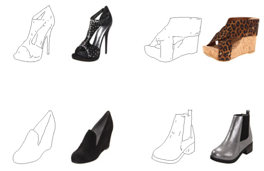
In this section, you will implement an image-to-image translation program based on pix2pix. You will train the pix2pix model on the edges2shoes dataset to translate images containing only the edges of a shoe, to a full image of a shoe. The edges are automatically extracted from the real shoe images. This section uses the notebook hw5_gan.ipynb.
Some example edge/image pairs are shown in Figure 1

The pix2pix model is based on a conditional GAN (Figure 2). The generator G maps the source image x to a synthesized target image. The discriminator takes both the source image and predicted target image as its inputs, and predicts whether the input is real or fake.
Task 1: Dataloading
You will first build data loaders for training and testing. For the training, you can use a batch size of 4. During testing, you will process 5 images in a single batch, so that we can visualize several results at once.
Task 1.1: (5 points) Implement the Edges2Image class and fill in the TODOs in that cell.
Hint: please use the DataLoader from torch.utils.data
We have provided the implementation for the generator and the discriminator models in the notebook. Refer and familiarize yourself with the architecture from the model summary, especially the input and the output shapes.
Task 2: Training Pix2Pix
Optimization
- For optimization, we’ll use the Adam optimizer. Adam is similar to SGD with momentum, but it also contains an adaptive learning rate for each model parameter. If you want to learn more about Adam, please refer to the deep learning book by Ian Goodfellow et al. For our model training, we will use a learning rate of 0.0002, and momentum parameters β1 = 0.5 and β2 = 0.999.
Task 2.1: (5 points) Please set up G_optimizer and D_optimizer in the train function.
Pix2Pix Objective Function
Given a generator \(G\) and a discriminiator \(D\), the loss function / objective functions to be minimized are given by
\[\mathcal{L}_{cGAN}(G, D) = \frac{1}{N} \left(\: \sum_{i=1}^{N} log D(x_i, y_i) + \sum_{i=1}^{N} log (1 - D\:(x_i, \:G\:(x_i)) \:) \right)\]where \((x_i, y_i)\) refers to the pair to the ground-truth input-output pair and \(G(x_i)\) refers to the image translated by the Generator.
\[\mathcal{L}_{L1}(G, D) = \frac{1}{N} \sum_{i=1}^{N} \|\:y - G(x_i) \:\|_1\]The final objective is just a combination of these objectives.
\[\mathcal{L}_{final}(G, D) = \mathcal{L}_{cGAN}(G, D) + λ \:\mathcal{L}_{L1}(G, D)\] \[G^* = \underset{G}{\mathrm{argmin}} \:\underset{D}{\mathrm{max}}\; \mathcal{L}_{final}(G, D)\]You would be implementing these objectives using the nn.BCELoss and nn.L1Loss as provided in the code.
Task 2.2: (10 points) Implement the code for the function train as instructed by the notebook.
- You will train the model using the objective \(\mathcal{L}_{final}\) using λ = 100. Train the network for at least 20 epochs. You are welcome to train longer, though, to potentially obtain better results. Please complete the following tasks for the report.
- Attach the plot for the history of the Discriminiator.
- Attach the plot for the history of the BCE Loss of the Generator.
- Attach the plot for the history of the L1 Loss of the Generator.
Task 2.3: (5 points) In your report, include these plots.
Section 2: Diffusion Models
In this section, you will be exploring various diffusion-based sampling algorithms using a pre-trained diffusion model. We will be focusing on two kinds of problems in this section. This section uses the notebook hw5_diffusion.ipynb and the python files guided_diffusion/simple_diffusion.py and guided_diffusion/condition_methods.py.
Download the model weights file ffhq_10M.pt and upload this file to the models/ directory.
- Uncondiional Sampling : This refers to generating randomly sampled images using diffusion sampling. You would be usinga pre-trained diffusion model trained on the FFHQ dataset.
- Image Inpainting: This refers to completing unknown regions in an image by conditionally sampling a diffusion model.
Specifically, we would be having four tasks for this section.
- Denoising Diffusion Probablistic Models (DDPM)
- Denoising Diffusion Implicit Models (DDIM)
- Inpainting using DDPMs (Repaint)
- Diffusion Posterior Sampling (DPS)
You are free to read these papers for an in-depth understanding of these algorithms, however, for the scope of this assignment, we suggest you to refer the lecture slides.
Unconditional Sampling using DDPM
Implementing Linear and Cosine Schedule
Diffusion models are trained by adding a known amount of noise to a clean image and then apply iterative denoising to reconstruct this image. The amount of noise added (noise variance) at each step (a ‘timestep’ from here on) is determined by a schedule. In this task, you will be implementing two scheduling functions. Follow the instructions in the notebook to create a linear and a cosine scheduler for noise variances.
Using the schedule, for any timestep \(t\), noise is added to a clean image \(x_0\) to get a noisy image \(x_t\) using the rule
\[x_t = \sqrt{1 - \beta_t}\: x_{t-1} + \sqrt{\beta_t}\: \epsilon \quad \text{where} \quad \epsilon \sim \mathcal{N}(0, \mathbb{I}) \quad \text{and} \quad t = 0,1,2,\dots T-1\]or, by using some math,
\[x_t = \sqrt{\bar{\alpha}_t}\: x_{0} + \sqrt{1 - \bar{\alpha}_t}\: \epsilon \quad \text{where} \quad \epsilon \sim \mathcal{N}(0, \mathbb{I})\]where \(\alpha_t = 1 - \beta_t\) and,
\[\bar{\alpha}_t = \prod_{s=1}^{t} \alpha_s\]In DDPM setting, we use \(T = 1000\) to ensure that the denoising process is roughly Gaussian. The code uses the following naming conventions.
betas: \({\beta_t}\) for \(t = 0,1,2,...,T-1\)alphas: \({\alpha_t}\) for \(t = 0,1,2,...,T-1\)alphas_cumprod: \({\bar{\alpha}_t}\) for \(t = 0,1,2,...,T-1\)
Task 3.1: (10 points) Implement the method get_named_beta_schedule with linear and cosine schedules.
DDPM Sampling: Iterative Denoising
In this step, you will be implementing the unconditional sampling on a pre-trained diffusion model. In its core, the diffusion model is a denoising model that accepts a noisy input \(x_t\) and predicts the noise that was added to the image \(x_0\) in the first place. We denote the model in the subsequent sections as \(\epsilon_{\theta}^{(t)}\) and model in the code.
In the code, you can get the predicted noise for any noisy image noisy at a timestep t using the call model(noisy, t).
Given the prediction of the model \(\epsilon_{\theta}^{(t)}(x_t, t)\), we can predict the clean image using the formula
\[\hat{x}_0 = \frac{x_t - \sqrt{1 - \bar{\alpha}_t} \: \cdot \epsilon_{\theta}^{(t)}(x_t, t)}{\sqrt{\bar{\alpha}_t}}\]Follow the instructions in the notebook and the class DDPMDiffusion in the code file guided_diffusion/simple_diffusion.py and implement the unconditional sampling using the pre-trained diffusion model to generate a sample.
Task 4.1: (10 points) Fill the TODO sections of the class DDPMDiffusion of the file guided_diffusion/simple_diffusion.py. Complete the methods p_sample and p_sample_loop.
Task 4.2: (5 points) In your report, include the generated sample.
Unconditional Sampling using DDIM
In this task, you will implement an improved sampling algorithm from Denoising Diffusion Implicit Models(DDPM) paper. DDIM sampling applies an improved update rule that helps to skip a few timsteps. The update rule is given by
\[x_{t-1} = \sqrt{\bar{\alpha}_{t-1}} \underbrace{ \left( \frac{x_t - \sqrt{1 - \bar{\alpha}_{t}}\: \epsilon_{\theta}^{(t)}(x_t)}{\sqrt{\bar{\alpha}_{t}}} \right) }_{\text{"predicted } x_0 \text{"}} + \underbrace{ \sqrt{1 - \bar{\alpha}_{t-1} - \sigma_t^2} \cdot \epsilon_{\theta}^{(t)}(x_t) }_{\text{direction pointing to } x_t } + \underbrace{ \sigma_t \epsilon_t}_{\text{random noise}}\]where
\[\sigma_{t}(\eta) = \eta \sqrt{\frac{1 - \bar{\alpha}_{t - 1}}{1 - \bar{\alpha_{t}}}}\: \sqrt{1 - \frac{\bar{\alpha_{t}}}{\bar{\alpha}_{t-1}}}\]Setting \(\eta = 0\) gives deterministic sampling and setting \(\eta = 1\) gives DDPM sampling.
The DDIM algorithm you will be implementing can skip a few timsteps every often, resulting in fewer timesteps (say 50 or 100 timesteps) as compared to DDPM which uses 1000 timesteps. So when applying the denoising, don’t forget to use model(noisy, self._scale_timesteps(t)). Use \(\eta = 0\) in this case and 100 timesteps for denoising.
Using the update rule, implement the DDIM sampling step in the method p_sample of the class DDIMDiffusion from the file guided_diffusion/simple_diffusion.
Task 5.1: (10 points) Complete the TODO sections in the p_sample of the class DDIMDiffusion from the file guided_diffusion/simple_diffusion.
Task 5.2: (5 points) In your report, include the generated sample using DDIM sampling.
Image Inpainting using RePaint
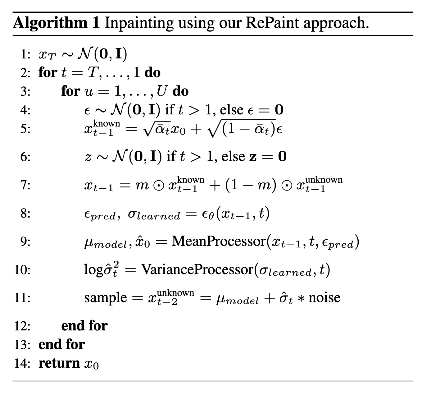
Repaint algorithm applies a repetitive denoising on the unknown regions of the image, thus allowing a generative fill. The core of the algorithm can be seen in Figure 3.

Follow the instructions from the notebook and the python files to implement an inpaiting step using the method p_sample of the class Repaint in guided_diffusion/simple_diffusion.py. Make use of one of the images and masks in the folder named data/datasets/ to simulate the inpaiting problem.
Note: The folder data/datasets/gts/ consists of ground-truth images and data/datasets/gt_keep_masks/ consist of some masks which you can use.
Task 6.1: (15 points) Fill the TODO sections of the class Repaint of the file guided_diffusion/simple_diffusion.py.
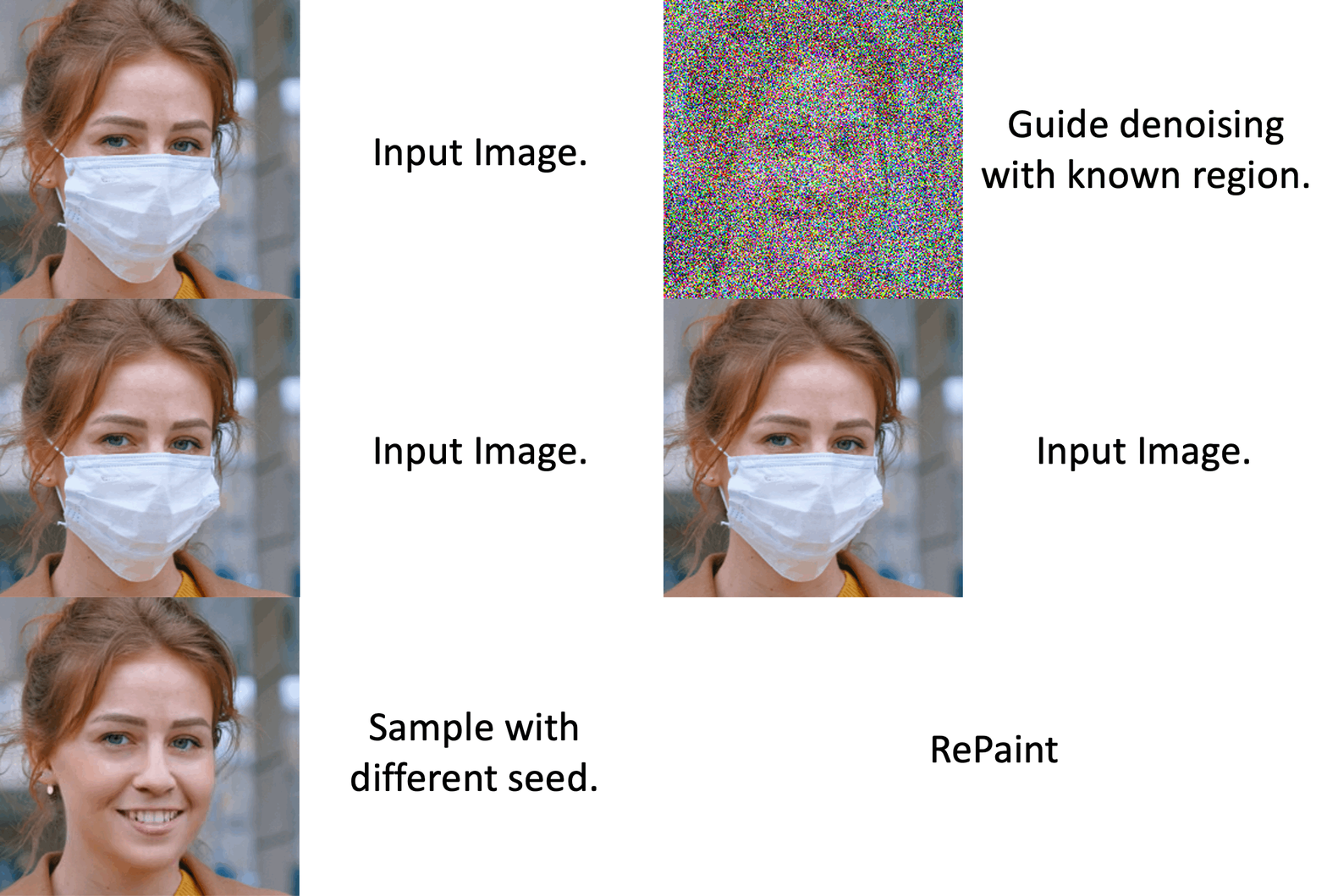
Task 6.2: (5 points) In your report, include the inpainted using Repaint.
You may expect the output to be similar to one of these inpainted figures in Figure 5.

Image Inpainting using Diffusion Posterior Sampling
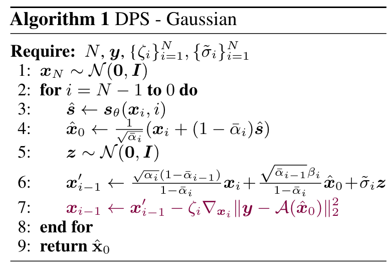
Diffusion Posterior Sampling (DPS) is another method for solving general inverse problem (inpaiting being an inverse problem itself). Refer to the algorithm in the Figure 5.

Follow the instructions in the notebook and the python files to implement the algorithm for diffusion posterior sampling.
Task 7.1: (10 points) Fill the TODO sections of the class PosteriorSampling of the file guided_diffusion/condition_methods.py. Hint: In practice \(\xi_i\) is usually set to be proportional to \(1/ \lVert \boldsymbol{y}-\mathcal{A}(\hat{\boldsymbol{x}}_0)\rVert\) as \(\hat{\zeta_i}/\lVert \boldsymbol{y}-\mathcal{A}(\hat{\boldsymbol{x}}_0)\rVert\) where \(\hat{\zeta_i}\) is a scalar independent of \(1/\lVert\boldsymbol{y}-\mathcal{A}(\hat{\boldsymbol{x}}_0)\rVert\). So line 7 in the algorithm can be re-writtent as \(x_{i-1} \leftarrow x_{i-1}^{\prime}-\hat{\zeta}_i\nabla_{\boldsymbol{x}_i}\lVert \boldsymbol{y}-\mathcal{A}(\hat{x}_0) \rVert_2\). In other works, you only need to take the gradient over the norm term, instead of the squared norm in our homework.
Task 7.2: (5 points) In your report, include the inpainted using DPS sampling.
Optional task for DPS
Play around with other task configurations and operate the algorithm to see how the results look like. Report one sample(including the raw image, corrupted image input and the algorithm output) of the following task: motion deblur, gaussain deblur and super resolution. Compare the results and discuss how the algorithm perform in each task. Hint: Change task_config to paly with different tasks
Tasks Checklist
This section is meant to help you keep track of the many things that go in the report:
- Dataloading:
- 1.1 - Dataloading
- Training Pix2Pix:
- 2.1 -
G_optimizerandD_optimizer - 2.2 -
trainfunction - 2.3 - Plots for discriminator and generator losses
- 2.1 -
- Implementing Linear and Cosine Schedule:
- 3.1 -
get_named_beta_scheule
- 3.1 -
- DDPM Sampling: Iterative Denoising:
- 4.1 -
p_sampleandp_sample_loopof classDDPMDiffusion - 4.2 - Sampled Image
- 4.1 -
- Unconditional Sampling using DDIM:
- 5.1 -
p_sampleof classDDIMDiffusion - 5.2 - Sampled Image
- 5.1 -
- Image Inpainting using RePaint:
- 6.1 -
p_sampleof classRepaint - 6.2 - Inpainted Image
- 6.1 -
- Image Inpainting using DPS:
- 7.1 -
PosteriorSampling - 7.2 - Inpainted Image
- 7.1 -
Canvas Submission Checklist
In the zip file you submit to Canvas, the directory named after your uniqname should include the following files:
- Python files:
simple_diffusion.pycondition_methods.py
- Notebooks:
hw5_gan.ipynbhw5_diffusion.ipynb
All plots should be included in your pdf report submitted to Gradescope. Run all the cells of your Colab notebooks, and do not clear out the outputs before submitting. You will only get credit for code that has been run.