EECS 442: Computer Vision (Winter 2024)
Homework 6 – 3D Deep Learning
Instructions
This homework is due at 11:59 p.m. on Wednesday April 17th, 2024.
The submission includes two parts:
-
To Canvas: submit a
zipfile containing a single directory with your uniqname as the name that contains all your code and anything else asked for on the Canvas Submission Checklist. Don’t add unnecessary files or directories.- We have indicated questions where you have to do something in code in red. If Gradescope asks for it, also submit your code in the report with the formatting below. Please include the code in your gradescope submission.
Starter code is given to you on Canvas under the “Homework 6” assignment. You can also download it here. Clean up your submission to include only the necessary files. Pay close attention to filenames for autograding purposes.
Submission Tip: Use the Tasks Checklist and Canvas Submission Checklist at the end of this homework.
-
To Gradescope: submit a
pdffile as your write-up, including your answers to all the questions and key choices you made.- We have indicated questions where you have to do something in the report in green. For coding questions please include in the code in the report.
The write-up must be an electronic version. No handwriting, including plotting questions. \(\LaTeX\) is recommended but not mandatory.
For including code, do not use screenshots. Generate a PDF using a tool like this or using this Overleaf LaTeX template. If this PDF contains only code, be sure to append it to the end of your report and match the questions carefully on Gradescope.
NERF:
-
You’ll be writing the code in the same way you’ve been writing for Homework 4 Part 2, i.e., Google Colab. You may use local Jupyter Notebooks, however suggest that you use Google Colab, as running these models on local system may consume too much of GPU RAM (This assignment is not CPU Friendly like Homework 4.).
-
We suggest you follow these steps to setup the codebase for this assignment depending on whether you are using Google Colab or your local system.
Google Colab: Steps to Setup the Codebase
- Download and extract the zip file.
- Upload the folder containing the entire code (with the notebook) to your Google Drive.
- Ensure that you are using the GPU session by using the
Runtime -> Change Runtime Typeand selectingPython3andT4 GPU. Start the session by clickingConnectat the top right. The default T4 GPU should suffice for you to complete this assignment.
Local System: Steps to Setup the Codebase
- Download and extract the zip file to your local directory.
- Get rid of the command lines that is specfic for google colabs.
- You are good to start Section 2 of the assignment.
Python Environment
The autograder uses Python 3.7. Consider referring to the Python standard library docs when you have questions about Python utilties.
To make your life easier, we recommend you to install the latest Anaconda for Python 3.7. This is a Python package manager that includes most of the modules you need for this course. We will make use of the following packages extensively in this course:


Estimation of the Fundamental Matrix and Epipoles
Data: we give you a series of datasets that are nicely bundled in the folder task1/. Each dataset contains two images img1.png and img2.png and a numpy file data.npz containing a whole bunch of variables. The script task1.py shows how to load the data.
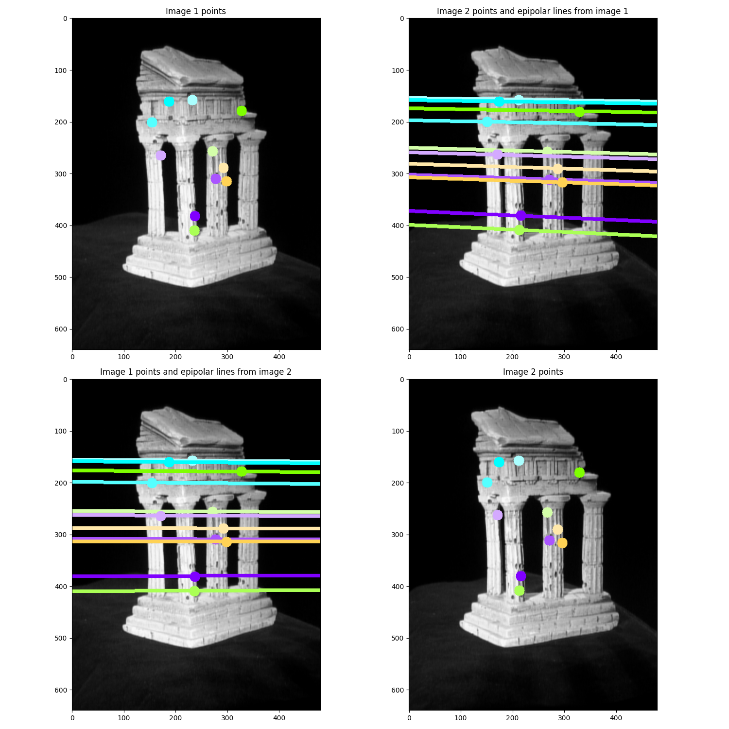
Credit: temple comes from Middlebury’s Multiview Stereo dataset.
Task 1: Estimating \(\FB\) and Epipoles
-
(15 points) Fill in
find_fundamental_matrixintask1.py. You should implement the eight-point algorithm mentioned in the lecture. Remember to normalize the data and to reduce the rank of \(\FB\). For normalization, you can scale the image size and center the data at 0. We want you to “estimate” the fundamental matrix here so it’s ok for your result to be slighly off from the opencv implementation. -
(10 points) Fill in
compute_epipoles. This should return the homogeneous coordinates of the epipoles – remember they can be infinitely far away! For computing the nullspace of F, using SVD would be helpful! -
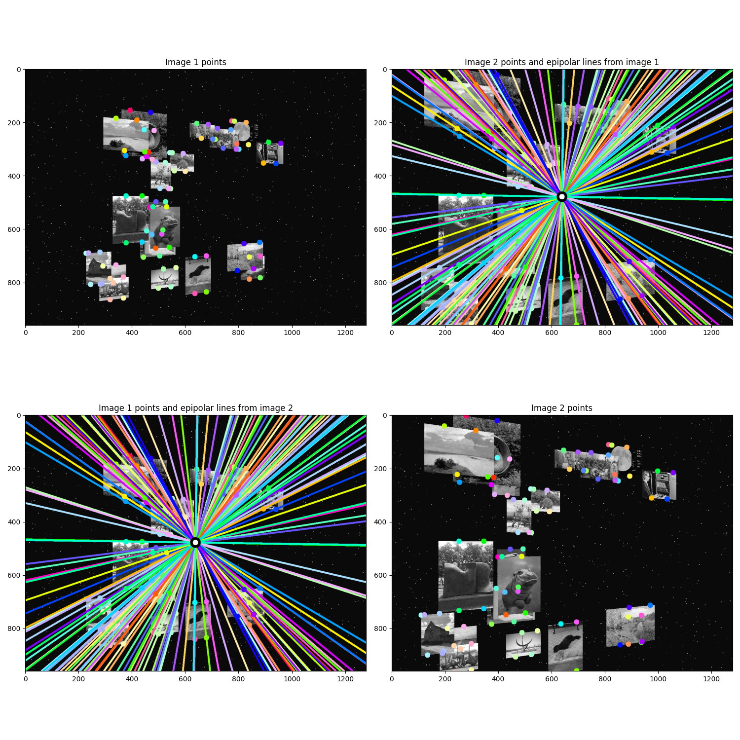
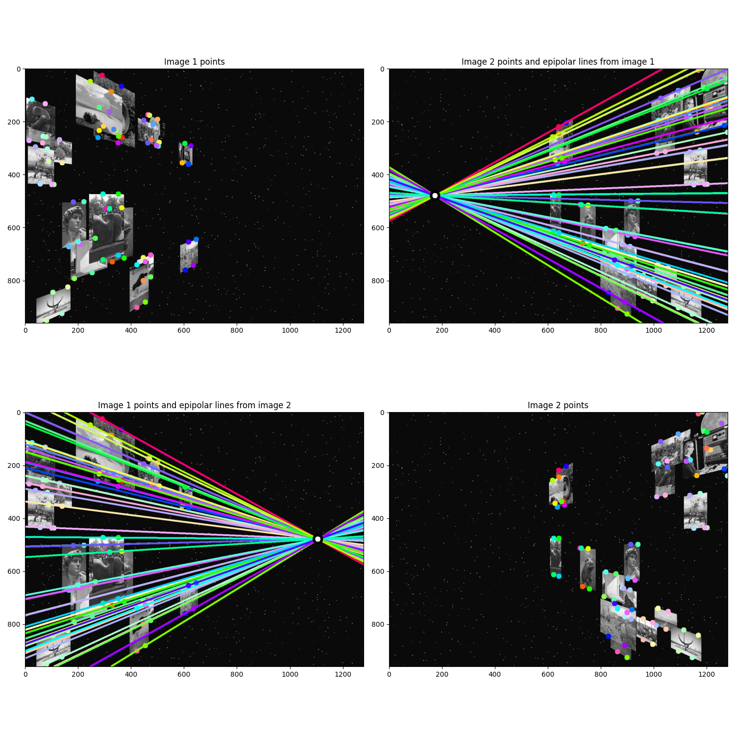
(5 points) Show epipolar lines for
temple,reallyInwards, and another dataset of your choice. -
(5 points) Report the epipoles for
reallyInwardsandxtrans.
3D Generation
Task 2: Neural radiance fields
We will fit a neural radiance field (NeRF) to a collection of photos (with their camera pose), and use it to render a scene from different (previously unseen) viewpoints. To estimate the color of a pixel, we will estimate the 3D ray that exist the pixel. Then, we will walk in the direction of the ray and query the network at each point. Finally, we will use volume rendering to obtain the pixel’s RGB color, thereby accounting for occlusion.
It is an MLP \(F_\Theta\) such that
\[F_\Theta(x, y, z, \theta, \phi) = (R, G, B, \sigma)\]where \((x, y, z)\) is a 3D point in the scene, and \((\theta, \phi)\) is a viewing direction. It returns a color \((R, G, B)\) and a (non-negative) density \(( \sigma)\) that indicates whether this point in space is occupied.
-
(10 points) Implement the function positional_encoder(x, L_embed = 6) that encodes the input x as \(\gamma(x) = (x, \sin(2^{0}x), \cos(2^{0}x), \ldots, \sin(2^{L_{embed}-1}x), \cos(2^{L_{embed}-1}x)).\)
-
(10 points) Implement the code that samples 3D points along a ray in
render. This will be used to march along the ray and query \(F_\Theta\) -
(10 points) After having walked along the ray and queried \(F_\Theta\) at each point in
render, we will estimate the pixel’s color, represented as rgb_map. We will also compute, depth_map, which indicates the depth of the nearest surface at this pixel. -
(10 points) Please implement part of the
train(model, optimizer, n_iters)function. In the training loop, the model is trained to fit one image randomly picked from the dataset at each iteration. You need to tune the near and far point parameter in get rays to make maximize the clarity of the RGB prediction image -
(5 points) Please include the best picture (after parameter tuning) of your RGB prediction, depth prediction, and groud truth figure for different view points.
We can now render the NeRF from different viewpoints. The predicted image should be pretty similar to the ground truth but it may have less clarity.
Tasks Checklist
This section is meant to help you keep track of the many things that go in the report:
- Estimating \(F\) and Epipoles
- 1.1 -
find_fundamental_matrix - 1.2 -
compute_epipoles - 1.3 - Epipolar lines for
temple,reallyInwards, and your choice - 1.4 - Epipoles for
reallyInwardsandxtrans
- 1.1 -
- Neural radiance fields
- 2.1 - Implement
positional_encoder - 2.2 - Sample 3D points along a ray
- 2.3 - Estimate
rgb_mapanddepth_map - 2.4 -
train - 2.5 - Report your prediction and groud truth image
- 2.1 - Implement
Canvas Submission Checklist
In the zip file you submit to Canvas, the directory named after your uniqname should include the following files:
task1.pyHW6_Neural_Radiance_Fields.ipynb